Table of Contents
- TL;DR
- The Setup
- A Few Terms
- Why Not Just Predict A Price?
- The Right Question
- Building The Acceptance Model
- From Probabilities To Prices: The Candidate Grid
- The Ladder Problem
- Solving The Ladder
- The Weighting Dial
- Where The Model Lives
- Evaluating The System
- The Gap Between Theory And Reality
- What Comes Next
- Closing
- Resources
Pricing looks like a prediction problem until you try to ship it.
The obvious question is: “what price will this customer accept?” Train a model, predict a number, serve it. Done.
Except that is the wrong level of abstraction. In practice, the useful question is: “for every price we are allowed to offer, what is $P(\text{accept} \mid p)$, and which price should we choose under the business constraints?”
That framing turns pricing from a single-number prediction problem into a decision problem. The model estimates behaviour. A separate optimisation layer chooses the action. A constraint layer makes sure the action is commercially safe.
This post walks through that system in the context of broadband regrade pricing: customers moving between product tiers, prices being recommended in real time, and the messy reality that the mathematically clean answer still has to survive business rules, price floors, product ladders, locked offers, and evaluation uncertainty.
TL;DR
- Do not train a model to predict the “right price” directly. Train it to estimate $P(\text{accept} \mid p)$ as a function of price.
- Once you have an acceptance curve, price selection becomes an explicit expected-value optimisation problem.
- The hard part is not just the model. It is the constraint system around it: floors, ceilings, product hierarchy rules, current-price anchors, pricing tiers, locked offers, and evaluation.
- The production design is modular: model for probabilities, optimiser for candidate selection, ladder module for coherence, and evaluation engine for counterfactual impact.
- In production, operational constraints can compress the model’s freedom so much that the theoretical uplift becomes small and volatile. That is not necessarily a modelling failure. It is a system design reality.
The Setup
Imagine you run a broadband business. You have millions of customers on different plans. Some are in contract, some are out of contract, some are close to renewal, and some are likely to churn. Every day, a subset of them enter a regrade journey: they consider switching to another product in the portfolio while staying with the same provider.
At that point, the business has to answer a practical question: what price should we show?
It is tempting to treat this as a regression task. Take customer features, product features, channel features, and historical pricing data, then predict a price. That sounds simple enough.
The problem is that pricing is not just prediction. It is prediction plus choice under constraints.
If you predict one price, you have not said what trade-off you are making between acceptance probability and revenue. You have not said whether you are willing to lose a little conversion for a higher monthly price. You have not said how to handle a faster product being accidentally cheaper than a slower product. You have not said what happens if the customer’s current product is priced above what they already pay.
Those are not modelling details. They are the actual decision.
A Few Terms
Before getting into the mechanics, here are the pieces of vocabulary that matter.
| Term | What it means |
|---|---|
| Regrade | A customer switching from one broadband product to another, such as upgrading speed or changing bundle, while staying with the same provider. |
| ARPU | Average Revenue Per User: the monthly recurring charge a customer pays. |
| ARPU delta | The change in monthly revenue when a customer regrades. It is often negative because regrades frequently involve a price reduction to retain the customer. |
| Floor / ceiling | The minimum and maximum allowed in-contract price for a product. These are business configuration values, not model outputs. |
| Product hierarchy | Products ranked by speed or value, for example 100Mbps, 300Mbps, 500Mbps, then Gigabit. A product’s position determines its hierarchy level. |
| Ladder | The full set of prices across hierarchy levels shown to a customer in one session. It must be internally coherent: higher hierarchy levels should not be cheaper than lower ones. |
| Pricing tier | A presentation slot determining offer priority. Tier 1 is the primary recommendation shown to the customer. The ML model generates prices for tier 1. |
| Session | A single customer interaction, such as a call centre call or web visit, where multiple product options can be shown. One session corresponds to one pricing decision context. |
| Churn | A customer leaving the provider entirely: the outcome the system is trying to prevent. |
| Locked offer | A manually-set incentive price, usually for customers near contract end, that overrides model recommendations. |
Why Not Just Predict A Price?
The most natural first instinct is to train a regression model on historical accepted prices.
customer, product, channel, context -> accepted_price
This fails for a subtle but important reason: the model has no incentive structure.
It learns the average historical price associated with acceptance. That price is not necessarily revenue-maximising. It is not necessarily conservative. It is not necessarily aligned with the business’s current risk appetite. It is just the average result of past decisions, with their biases, rules, overrides, and historical quirks baked in.
You can try to patch this after the fact. Cap the output. Floor it. Add a margin. Nudge certain segments up or down. But now the model is optimised for one objective and the decision layer is bending it toward another. Over time, the corrections stack up, interactions become hard to reason about, and nobody can clearly explain why a customer received a particular price.
That is a sign that the framing is wrong.
The Right Question
Instead of asking:
What price will this customer accept?
we ask:
For every possible price we could offer, what is the probability this customer would accept it?
For a given customer and product, the model estimates:
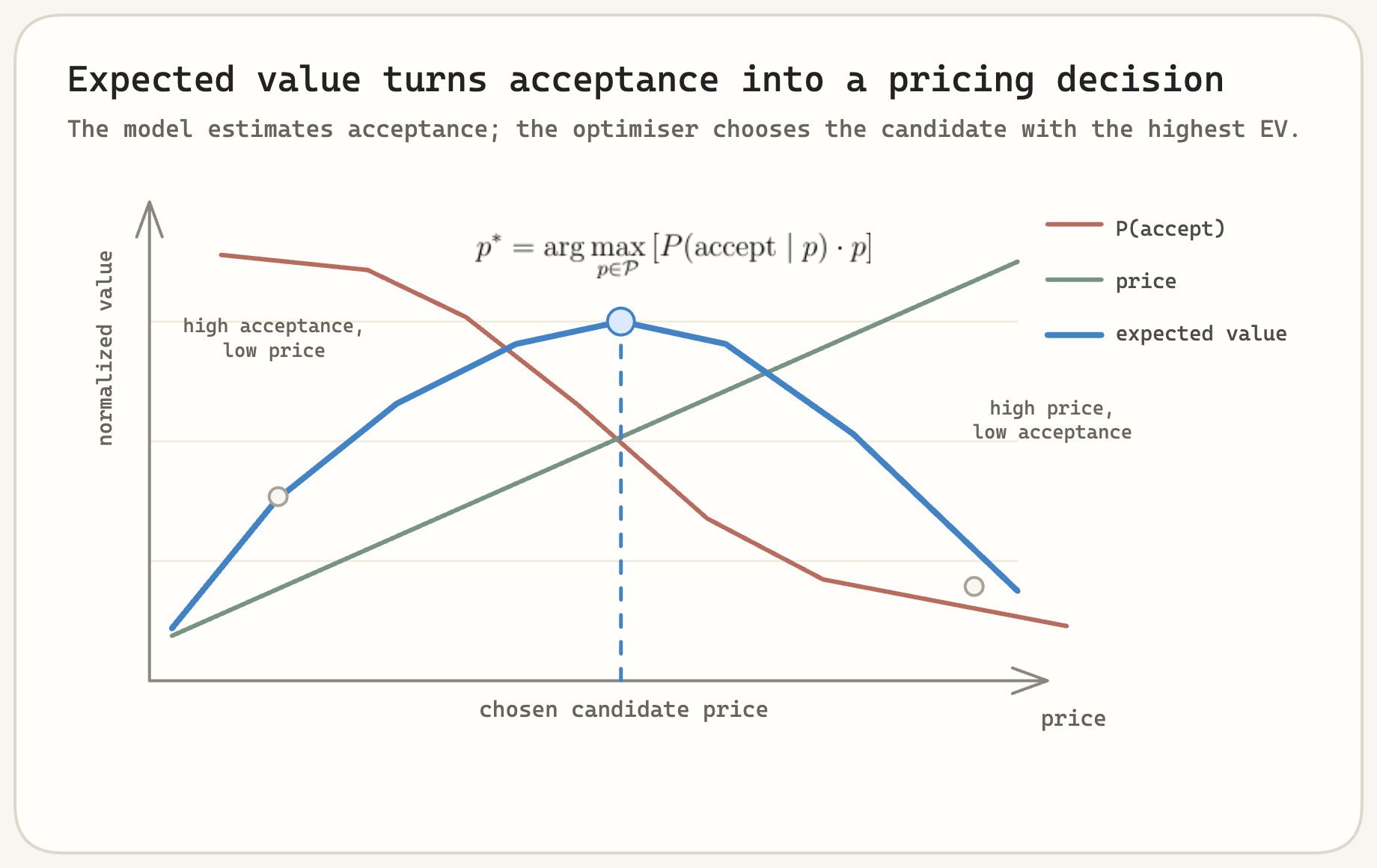
\[P(\text{accept} \mid \text{customer}, \text{product}, \text{channel}, p)\]That gives us an acceptance curve rather than a single price. Once you have that curve, the pricing decision becomes explicit. For each candidate price, compute expected value:
\[\operatorname{EV}(p) = P(\text{accept} \mid \text{customer}, \text{product}, p) \cdot p\]Then choose the candidate with the highest expected value, subject to the constraints the business cares about.
The key shift is separation of concerns. The model does not decide the price directly. The model estimates the probability of acceptance at each possible price. The optimiser decides which price to serve.
Building The Acceptance Model
The core model is an XGBoost binary classifier. Each training row represents a historical recommendation event: a customer was shown a product at a specific price, and we observe whether they accepted it.
The target is simple:
accepted_offer = 1 if the customer accepted, else 0
The important feature engineering choice is how price enters the model.
We do not feed raw price directly. Raw price is too product-specific. A price of £35 might be cheap for one product and expensive for another. Instead, we calculate a relative pricing signal:
discount = offered_price - average_historical_price_for_this_product
The average historical price is a rolling weighted mean of recently accepted prices for the same product and channel. It acts as a market anchor: the typical price customers have recently seen and accepted for that product.
The discount feature then answers a more useful question:
How far from normal is this offer?
If the discount is negative, the offer is cheaper than the recent market anchor. If it is positive, the offer is more expensive.
The Monotonic Constraint
There is one structural rule we want the model to respect:
As price increases relative to the market anchor, $P(\text{accept})$ should not increase.
In XGBoost, this can be expressed as a monotonic constraint on the discount feature. The model is allowed to learn nonlinear effects, interactions, and segment-specific behaviour, but it is not allowed to learn that making a product more expensive makes customers more likely to accept it.
This is more than regularisation. It is an economic invariant. A rational customer should not become more likely to accept the same product simply because it became more expensive relative to what similar customers have recently paid.
Without this constraint, the optimiser can become unstable. If the model has local bumps where a higher price appears to increase acceptance probability, the expected-value calculation may chase noise. A monotonic acceptance curve makes the downstream grid search much better behaved.
The full model used around 200 features, including:
- Pricing signals such as discount, ARPU deltas, and historical discount behaviour.
- Customer lifecycle signals such as tenure, contract status, and current product holdings.
- Geographic market signals such as local churn rates and competitive density.
- Behavioural signals such as call history, complaint flags, and sentiment.
- Channel and product encodings.
The model’s job is not to understand every business rule. Its job is narrower: estimate acceptance probability for a customer, product, channel, and candidate price.
Avoiding Session Leakage
There is one important trap in training: sessions contain multiple rows.
A single regrade session may show several products at several prices. If one row from a session lands in training and another lands in validation, the validation score is contaminated. The model has effectively seen part of the same customer decision context during training.
The fix is group-aware cross-validation, using session ID as the group. Every row from a session stays together.
session_123 rows -> training fold only
session_456 rows -> validation fold only
No split is allowed to break a session apart.
For Bayesian hyperparameter optimisation, we used TPE via Hyperopt. Early stopping was separated from cross-validation evaluation:
- Run early stopping once on a fixed held-out evaluation split.
- Use that split to choose
n_estimators. - Fix
n_estimators. - Run group-aware cross-validation without fold-specific early stopping.
That keeps trials comparable. Otherwise, each fold can stop at a different number of trees, adding noise to the hyperparameter search.
It is a small design choice, but it avoids a surprising amount of evaluation instability.
From Probabilities To Prices: The Candidate Grid
With an acceptance model in place, the decision layer can choose a price.
For each customer and product combination, the system evaluates a candidate grid:
- Generate 41 candidate prices from the average historical price, using
£1increments frombaseline - £20tobaseline + £20. - Apply commercial bounds by masking candidates below the product floor or above the product ceiling.
- Assign invalid candidates a score of $-\infty$ so they can never be selected.
- Repeat the customer’s features 41 times, append the candidate-specific discount value, and make one batched
predict_probacall. - Compute the score for every valid candidate.
- Select the candidate with the highest score.
The neutral expected-value score is:
\[\operatorname{score}(p) = P(\text{accept} \mid p) \cdot p\]In production, we also include a configurable weighting term:
\[\operatorname{score}(p) = P(\text{accept} \mid p) \cdot p \cdot (1 + w \cdot d)\]Here $d$ is the candidate’s discount feature and $w$ is the weighting value. The weighting function encodes risk preference. More on that shortly.
The important engineering detail is that this is vectorised. There is no iterative search and no per-price loop through the model. The entire local price curve is evaluated in one batch inference call.
That makes the pricing path fast enough for real-time recommendation while still letting the decision layer inspect the full local trade-off between acceptance probability and price.
The Ladder Problem
If the system priced one product at a time, the candidate grid would be enough. But regrade journeys usually show a menu of products at once.
Broadband products sit in a hierarchy, typically by speed or value: 100Mbps, 300Mbps, 500Mbps, Gigabit, and so on. That hierarchy creates a hard commercial rule:
A faster product must never be cheaper than a slower product.
The model does not know this rule. It optimises each customer-product pair independently. That means the raw optimal prices can look like this:
| Level | Product | Raw model price |
|---|---|---|
| 1 | 100Mbps | £32 |
| 2 | 300Mbps | £29 |
| 3 | 500Mbps | £41 |
The level 2 price is lower than level 1. That might be explainable from the model’s local expected-value surface, but it is incoherent as a customer-facing product ladder.
There is also a second hard rule:
The recommended price at the customer’s current tier must not exceed what they currently pay.
If someone is already on a product, you cannot frame “stay where you are but pay more” as a regrade recommendation. That is a price rise wearing a trench coat.
Each product also has its own floor and ceiling, and those bounds can conflict once prices have to be monotonic across the ladder. Tightening one tier can cascade into adjacent tiers.
This is where a deterministic constraint layer becomes necessary.
Solving The Ladder
The ladder module takes the model’s raw per-product optimal prices and makes them globally coherent.
It works in four stages.
Stage 1: Isotonic Smoothing
First, apply isotonic regression to find the closest non-decreasing sequence to the raw model prices.
In plain English: change the prices as little as possible while removing hierarchy violations.
For example:
raw prices:       £32, £29, £41, £44, £43
smoothed prices:  £30.5, £30.5, £41, £43.5, £43.5
The exact output depends on weights and implementation details, but the principle is the same. Isotonic regression gives a minimal-deviation monotonic sequence. It is a mathematically clean nudge rather than a hand-written patch.
Stage 2: Anchor The Current Tier
Next, tighten the ceiling at the customer’s current hierarchy level to their current price, rounded into the same commercial £X.99 format used for final offers.
If the customer currently pays £37.99 for level 2, then level 2’s ceiling becomes at most £37.99, even if the product’s general commercial ceiling is higher.
This prevents the system from recommending an increase at the current product level.
Stage 3: Propagate Bounds Across The Ladder
Local floors and ceilings are not enough. If level 3 has a floor of £40, then levels above it must also be at least £40 if the ladder is non-decreasing. If level 2 has a ceiling of £35, then levels below it must not exceed £35.
So the system converts local bounds into cumulative bounds:
\[\operatorname{cumulative\_floor}_i = \max(f_0, f_1, \ldots, f_i)\] \[\operatorname{cumulative\_ceiling}_i = \min(c_i, c_{i+1}, \ldots, c_n)\]If there are required price gaps between tiers, those step sizes are included in the cumulative calculation too.
The smoothed sequence is clipped into those cumulative bounds and checked for monotonicity again.
Stage 4: Commercial Formatting
Finally, prices are rounded to the required commercial format, such as £X.99.
This happens last. If formatting happens before constraint logic, rounding can create new hierarchy or floor/ceiling violations. The safe order is: optimise, smooth, constrain, then format.
The result is a price ladder that stays as close as possible to the model’s expected-value-optimal prices while being non-decreasing, floor/ceiling compliant, and anchored at the customer’s current tier.
In some edge cases, the constraints cannot all be satisfied at once. When that happens, the system prioritises commercial safety over marginal expected-value gains. It is better to leave a little revenue on the table than serve an incoherent or rule-violating ladder.
The Weighting Dial
The neutral score maximises expected value:
\[\operatorname{score}(p) = P(\text{accept} \mid p) \cdot p\]But pricing is rarely neutral in practice. Sometimes the business wants to be more conservative, especially for customers at risk of churn. Sometimes it wants to be more aggressive, especially where retention risk is low.
The system exposes this through a single weighting value:
\[\operatorname{score}(p) = P(\text{accept} \mid p) \cdot p \cdot (1 + w \cdot d)\]When $w = 0$, the system maximises raw expected value. When $w$ is negative, the score favours lower prices and becomes more conservative. When $w$ is positive, the score leans toward higher prices and becomes more aggressive.
This is useful because the risk preference is explicit. It is not hidden inside the model.
To tune it, we sweep the weighting value across a range for each customer segment. In this case, segments were defined by contract lifecycle stage and product type. For each value, we measure:
- Mean price adjustment.
- Mean predicted acceptance probability.
The result is a trade-off curve. As the weighting becomes more conservative, prices fall and predicted acceptance rises. But the relationship is not linear. There is usually a point where acceptance improves meaningfully with little revenue sacrifice, followed by a region where the business gives away margin for almost no additional acceptance.
Different segments have different curves. An out-of-contract customer in a competitive area may have a steep trade-off. A recently renewed customer in a less competitive area may be much flatter.
This is one of the cleanest parts of the design. The model estimates the acceptance curve. The weighting dial expresses business risk appetite. The two are connected, but not tangled together.
Where The Model Lives
The ML model is only one component in a larger pricing machine.
In simplified form, the production path looks like this:
That placement matters. The model does not see the whole product catalogue. It only sees products that have already survived filtering. It only generates prices for pricing tier 1, the primary recommendation. Its recommendation can still be overridden by a locked offer.
The product floor the model sees is also not a single simple number. It can be derived from multiple configuration layers:
- Target price settings for the product.
- Price bounds as a fallback.
- Regrade policies that can raise the floor but not lower it.
The final floor is the maximum of these sources. That is deliberate defence in depth. The business defines a safe window. The model optimises inside it. The ladder module ensures cross-product coherence. Locked offers provide a final manual override.
The probabilistic core is surrounded by deterministic safety layers.
Evaluating The System
Offline evaluation is hard because the historical data only tells us what happened at the prices that were actually offered. It does not directly tell us what would have happened if we had offered a different price.
To evaluate a new pricing strategy, we need counterfactual acceptance probabilities.
Counterfactual Acceptance Via The Three Regions
The evaluation framework uses a simple monotonic behavioural assumption within a single product offer:
- If a customer accepted price $A$, they would also have accepted any lower price $M < A$.
- If a customer rejected price $R$, they would also have rejected any higher price $M > R$.
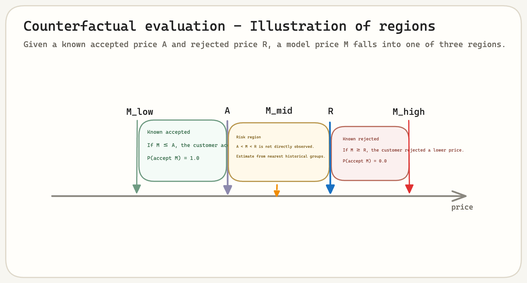
That gives us three regions for a model-recommended price $M$.
Region 1: Definitely Accepted
If the model recommends a price at or below a price the customer actually accepted, assign acceptance probability $1.0$.
\[M \le A \quad \Rightarrow \quad P(\text{accept } M) = 1.0\]We know the customer accepted a higher or equal price, so the lower model price would have been accepted too. The downside is that we may have left money on the table.
Region 2: Definitely Rejected
If the model recommends a price at or above a price the customer actually rejected, assign acceptance probability $0.0$.
\[M \ge R \quad \Rightarrow \quad P(\text{accept } M) = 0.0\]We know the customer rejected a lower or equal price, so the higher model price would not have worked.
Region 3: The Ambiguous Region
The ambiguous region is between known accepted and rejected prices. Here, we estimate acceptance probability from historical behaviour rather than using the model’s own prediction.
If the customer accepted at price $A$ and the model proposes a higher price $M$:
\[P(\text{accept } M) = \frac{P(X \ge M)}{P(X \ge A)}\]If the customer rejected at price $R$ and the model proposes a lower price $M$:
\[P(\text{accept } M) = 1 - \frac{1 - P(X \ge M)}{1 - P(X \ge R)}\]The probabilities come from nearest-match lookups in historical grouped data, using dimensions such as channel, product, and ARPU band.
The important point is that we do not evaluate the model using its own predictions. That would be circular. Instead, the evaluation engine uses rule-first logic where outcomes are known and historical nearest-neighbour grounding where they are not.
This is intentionally conservative: rules first, probability second, and no extrapolation beyond what the data can support.
Gain Decomposition
An average uplift number is not enough to understand a pricing system. You need to know what kind of uplift it is.
The three-region evaluation framework lets us decompose outcomes into four mutually exclusive categories:
| Category | Interpretation |
|---|---|
| Accepted + higher price | Pure upside: charged more and the customer still accepted. |
| Accepted + lower price | Underpriced: revenue left on the table. |
| Rejected + higher price | Overpriced: the customer walked away. |
| Rejected + lower price | Conservative but harmless: they were not going to accept anyway. |
For each category, gain is computed as:
\[\operatorname{gain} = \sum_i m_i \cdot \hat{q}_i - \sum_i b_i \cdot y_i\]Here $m_i$ is the model price, $\hat{q}_i$ is the counterfactual acceptance probability, $b_i$ is the baseline price, and $y_i$ is the observed transaction indicator.
This decomposition matters because two strategies can have the same average uplift for very different reasons.
One strategy might win by finding customers who tolerate higher prices. Another might win by converting previously lost customers with slightly lower offers. Those are different commercial stories, and they imply different next steps.
The Revenue Picture
Session-level gain is useful, but the business ultimately cares about total revenue impact across the base.
That means accounting for at least three macro effects.
| Effect | What it captures |
|---|---|
| ARPU delta investment | Lower prices mean larger monthly revenue sacrifice, multiplied across expected tenure. |
| Churn value lost | Each churn means lost contribution margin across the remaining customer lifetime. |
| Churn save value | Each save preserves lifetime value, net of regrade processing cost. |
The weighting parameter trades off between these effects.
An aggressive model extracts more revenue from customers who accept, but may save fewer customers at risk of churn. A conservative model may save more customers, but with a larger ARPU investment.
This is why the decision framing matters. The business is not really optimising model AUC or log loss. It is optimising a portfolio-level financial trade-off.
The Gap Between Theory And Reality
In isolation, this system is elegant. The acceptance model is calibrated around a useful economic signal. The expected-value optimisation is direct. The ladder enforcement is principled. The evaluation framework is conservative and auditable.
But production environments have opinions. Strong ones.
When we compare the ML strategy against other approaches, such as rule-based pricing, manual pricing, or control strategies, the differences in aggregate metrics are often small and volatile.
In one representative weekly readout, the ML-priced strategy had a higher regrade rate than the control, roughly 27% versus 25%, but also a slightly larger ARPU delta, roughly -£1.64 versus -£1.02. The net revenue impact was broadly comparable across strategies.
That is not failure, but it is humbling.
The operational constraints compress the model’s effective pricing freedom. The model may want to price at the peak of the expected-value curve, but after floors, ceilings, anchoring, locked offers, and tier restrictions, the served price can end up close to where a simpler heuristic would have landed anyway.
The main compression mechanisms were:
- Pricing tier restriction: ML pricing only generated prices for pricing tier 1.
- Floor ratcheting: Regrade policies pushed floors upward and narrowed the candidate grid from below.
- Locked offer overrides: High-value customers were often removed from the model’s control precisely where personalisation could matter most.
- Metric sensitivity: Weekly cohorts of a few thousand regrades produced wide confidence intervals.
This is an important lesson for production ML. Sometimes the bottleneck is not model quality. It is the amount of decision freedom the surrounding system gives the model.
What Comes Next
The next improvements are less about model sophistication and more about operational integration.
Useful next steps would be:
- Expand ML pricing beyond pricing tier 1 so the model can influence more of the product ladder.
- Revisit floor and ceiling configurations to make sure they reflect current market reality rather than historical conservatism.
- Find safe ways to apply personalised pricing to high-value customers currently handled by locked offers.
- Use longer evaluation windows to reduce weekly volatility and measure cumulative impact more reliably.
This is the unglamorous part of ML in production. The model can be ready before the organisation is ready to give it more room.
Closing that gap is not only an engineering problem. It is a trust problem. It requires evidence, stakeholder alignment, careful guardrails, and patience.
Closing
The thing I keep coming back to is the reframing.
“Predict the best price” gives you a regression problem with no explicit notion of trade-offs.
“Predict acceptance probability as a function of price” gives you a classification problem that enables explicit trade-off reasoning downstream.
The monotonic constraint is powerful because it encodes one simple economic assumption: making the offer more expensive should not make it more attractive. That one structural assumption makes the downstream optimisation much easier to reason about.
The ladder enforcement shows what happens when you take constraint satisfaction seriously. Instead of bolting rules onto the side of the model, the system defines a deterministic module whose only job is to make the price vector commercially coherent.
And the counterfactual evaluation approach has the right kind of humility. It uses certainty where the data gives certainty, estimates only in the ambiguous region, and avoids pretending the model can validate itself.
The broader lesson is the gap between what a model could do and what a system allows it to do. Closing that gap is less about algorithms and more about partnerships.
Resources
- XGBoost monotonic constraints - useful reference for encoding monotonic relationships directly into boosted tree models.
- scikit-learn IsotonicRegression - documentation for fitting a monotonic sequence with minimal deviation.
- scikit-learn GroupKFold - useful when rows are not independent and whole groups must stay together across train/validation splits.
- Hyperopt - a common Python library for Bayesian-style hyperparameter optimisation.