
Table of Contents
- What is XGBoost?
- Ok…so what are hyperparameters?
- How does tuning fit into this picture?
- A practical tuning recipe
- Useful Resources
XGBoost ships with dozens of “levers” you can pull, and the difference between a mediocre model and a strong one often comes down to how well you set them. This post walks through what those hyperparameters actually do, grouped by the part of the model they affect, and then works up the tuning ladder: from validation curves for a single parameter, to grid search, to Bayesian optimization with Hyperopt.
What is XGBoost?
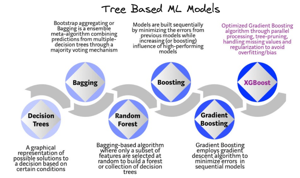
XGBoost, or eXtreme Gradient Boosting, can be thought of as a particular implementation of the gradient boosted trees algorithm, introduced by Tianqi Chen & Carlos Guestrin in their 2016 paper. It is open source and widely considered one of the best ML algorithms in the context of structured tabular data (in terms of performance, efficiency etc) even today.
Ok…so what are hyperparameters?
When applying algorithms to your data it’s often the case that they come with “levers” that you can fiddle with to alter the effectiveness of the algorithm on your specific problem. Formally speaking these levers are referred to as hyperparameters of your model and can have different optimal values depending on your data.
Note: These levers are separate to the inherent learned information of the model when you call the
.fit()method on your model object (assumingscikit-learnbased model APIs). These “levers” are not determined via the model learning process itself but rather trial and error, and are passed in as arguments to your model object’s constructor during instantiation (something likeXGBClassifier(**params)whereparamsis a dictionary object with keys corresponding to the hyperparameter names and values being the values they should take on).
In the case of XGBoost many hyperparameters exist so it’s important to know what they are and ways to classify them. A good way to do this is by grouping them by “what they impact”, in which case the following groupings apply:
Note: The list provided below is not exhaustive, more details can be found on the XGBoost parameters docs. A general observation is that when parameters contain the
max_prefix, increasing them causes a rise in complexity while reducing them causes an increase in simplicity. Parameters with themin_prefix have the opposite effect, whereby increasing them tends to simplify things and vice versa.
- Tree creation
- Ultimately XGBoost consists of trees so these params control the properties of those underlying trees.
- Parameters:
max_depth=6: Tree depth, how many feature interactions you can have. Larger is more complex (potential overfitting). The number of possible splits doubles at each level (imagine number of leaves i.e. $2^{n}$). It can take a range of values $n \in [0, \infty]$.max_leaves=0: Number of leaves in the tree. A larger number increases complexity. It can take a range of values $n \in [0, \infty]$.min_child_weight=1: Minimum sum of hessian (weight) needed in a child. A larger value is more conservative. It can take a range of values $n \in [0, \infty]$. This blog post contains more info.grow_policy='depthwise': Only supported withtree_methodset to ['hist', 'approx', 'gpu_hist']. Splits nodes closest to the root. Set to'lossguide'(withmax_depth=0) to mimic LightGBM behavior.tree_method='auto': Use'hist'to use histogram bucketing and increase performance.'auto'acts as a heuristic.'exact'for small data'approx'for larger data'hist'for histograms (limit bins withmax_bin, default 256)- In XGBoost 2.0+ GPU training moved to
device='cuda'combined withtree_method='hist', replacing the older'gpu_hist'.
- Sampling
- These affect the sampling procedure at various levels within the model, since subsets of columns are taken as part of the underlying model architecture. They tend to have compounding dependencies e.g. if
colsample_bytree = colsample_bylevel = colsample_bynode = 0.5then some nodes would see $(0.5)^{3} = 0.125$, i.e. $12.5\%$, of the initial columns. - Parameters:
colsample_bytree: Fraction of columns to be sampled for a tree (as a decimal). It can take a range of values $n \in (0, 1]$ however the searching recommendation is $[0.5, 1]$.colsample_bylevel: Fraction of columns to be sampled for a level inside a tree (as a decimal). It can take a range of values $n \in (0, 1]$ however the searching recommendation is $[0.5, 1]$.colsample_bynode: Fraction of columns to be sampled at each node split (as a decimal). It can take a range of values $n \in (0, 1]$ however the searching recommendation is $[0.5, 1]$.subsample: Proportion of training data rows sampled prior to each successive boosting round. Lower is more conservative and reduces computation. It can take a range of values $n \in (0, 1]$ however the searching recommendation is $[0.5, 1]$. Setting $n < 1$ gives you stochastic gradient boosting, injecting a fair amount of randomness into the optimization, which often acts as a useful regularizer.sampling_method: How rows are sampled forsubsample.'uniform'gives every training row an equal probability of being selected;'gradient_based'(GPU training only) preferentially keeps rows with large gradients.
- These affect the sampling procedure at various levels within the model, since subsets of columns are taken as part of the underlying model architecture. They tend to have compounding dependencies e.g. if
- Categorical data
- The XGBoost constructor has to have the argument
enable_categorical=Trueset and the pandas DataFrame columns have to haveastype('category')where applicable for this to work. - Parameters:
max_cat_to_onehot=4: Upper threshold for using one-hot encoding for categorical features. One-hot encoding is used on categorical features when the number of categories present is less than this number.max_cat_threshold=64: Maximum number of categories to be considered for each split. A rough heuristic suggests $64$ for this.
- The XGBoost constructor has to have the argument
- Ensembling
- These parameters control how the subsequent trees are created and “ensembled”.
- Parameters:
n_estimators=100: Number of trees. A larger value will increase complexity. Useearly_stopping_roundsto prevent overfitting. You don’t really need to tune this if you useearly_stopping_rounds.early_stopping_rounds=None: Number of rounds after which you stop creating new trees if theeval_metricscore hasn’t improved. It can take a range of values $n \in [1, \infty]$.eval_metric: Chosen metric for evaluating validation data and the early stopping criteria. Classification metrics include ['logloss', 'auc'] whereas regression includes things like ['mae', 'rmse', 'rmsle', 'mape'].objective: Learning objective while fitting your model to the data during the training process. For classification this is either'binary:logistic'or'multi:softmax'/'multi:softprob'depending on whether it’s a binary or multi-class problem.
- Regularization
- Controls the complexity of the overall model, penalizing complexity to improve generalization.
- Parameters:
learning_rate=0.3: After each boosting round you shrink the contribution of the newly added tree to make the ensemble more conservative (the amount you want to move the predictions after each round). A lower value represents a more conservative impact. It can take a range of values $n \in (0, 1]$ and you typically lower this if you want to increasen_estimators.gamma=0/min_split_loss: Effectively L0 regularization. Minimum loss reduction required to split a leaf node. Effectively prunes the tree to remove splits that don’t meet the given value. A larger value is more conservative and it can take a range of values $n \in [0, \infty)$ where $n=0$ represents no regularization. The recommended search is over orders of magnitude, e.g. $(0, 1, 10, 100, 1000)$.reg_alpha=0: Effectively L1 regularization. Adds a penalty proportional to the sum of the absolute leaf weights to the loss, i.e. $\alpha \sum_{i=1}^{n} \lvert w_{i} \rvert$ where $w_{i}$ are the leaf weights. Increase this to be more conservative. It can take a range of values $n \in [0, \infty)$.reg_lambda=1: Effectively L2 regularization. Adds a penalty proportional to the sum of the squared leaf weights to the loss, i.e. $\lambda \sum_{i=1}^{n} w_{i}^{2}$ where $w_{i}$ are the leaf weights. Increase this to be more conservative. It can take a range of values $n \in [0, \infty)$.
- Imbalanced data
- Useful when your data distribution is imbalanced.
- Parameters:
scale_pos_weight=1: Consider the proportion $\frac{\text{count(negative)}}{\text{count(positive)}}$ for imbalanced classes. It can take a range of values $n \in (0, \text{large number})$.max_delta_step=0: Maximum delta step for leaf output. Can potentially help for imbalanced classes. It can take a range of values $n \in [0, \infty)$.
You can then view the hyperparameters for your model by doing something like:
import xgboost as xgb

# Create a dictionary of hyperparameters
params = {'objective': 'binary:logistic',
          'random_state': 42,
          'reg_alpha': 0,
          'reg_lambda': 1,
          'learning_rate': 0.1,
          }
xgb_classifier = xgb.XGBClassifier(**params)
xgb_classifier.fit(X_train, y_train)

xgb_classifier.get_params()  # This method returns all parameters for your model object
How does tuning fit into this picture?
The whole concept then of “hyperparameter tuning” is the process of trying to find the optimal values that the hyperparameters should take for your given problem.
There is no hard and fast rule for this and typical approaches tend to boil down to using techniques (some more complex than others e.g. GridSearch vs BayesianOptimization) to try a bunch of values, measure how the performance of your model changes as you vary those values, and finally settle on the set of values which provides the highest performance on your given data.
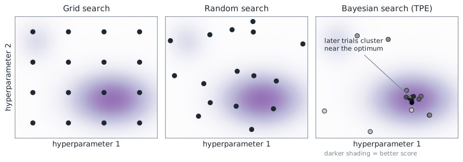
Before diving into code it’s worth having a picture of how the main search strategies differ, because they all answer the same question (“where should I evaluate next?”) in different ways:
- Grid search evaluates every combination of a fixed lattice of values. Exhaustive but expensive, and the cost explodes combinatorially as you add parameters.
- Random search samples combinations at random. For the same budget it tends to beat grid search in higher dimensions, because it doesn’t waste evaluations repeating the same few values of each individual parameter.
- Bayesian optimization (what Hyperopt does) uses the results of past trials to decide where to look next, spending most of its budget in the promising regions of the space.
Example: Single parameter tuning
Note: In practice this isn’t something you’d tend to do, but it is useful for demonstration purposes and for building intuition about a parameter you don’t understand.
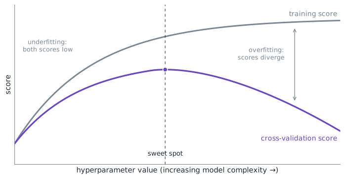
The key here is to use validation curves to plot your performance metric against your single hyperparameter and choose the hyperparameter value which yields the optimal performance. By keeping all other things constant you can attribute changes in performance as relating to that single hyperparameter.
In code this would look something like:
from yellowbrick.model_selection import validation_curve
import matplotlib.pyplot as plt
import xgboost as xgb

fig, ax = plt.subplots(figsize=(8, 4))
viz = validation_curve(
    xgb.XGBClassifier(n_estimators=200),
    X_train,
    y_train,
    param_name='gamma',
    param_range=[0, 0.5, 1, 5, 10, 20, 30],
    cv=5,
    scoring='roc_auc',
    ax=ax,
)
Where we have made use of the yellowbrick library’s validation curve functionality to plot and specified the necessary arguments including our estimator along with our dataset and the number of k-folds we want performed on our data to calculate our metric. For further details on cross-validation techniques check out scikit-learn’s docs.
Example: Using GridSearchCV for tuning
Calibrating individual hyperparameters takes some time and it can be difficult to know which combination is best. A potential solution to this is to select a group of hyperparameters that you want to tune and specify a set of values for each which can be searched together. You can make use of scikit-learn’s GridSearchCV for this.
import xgboost as xgb
from sklearn import model_selection

N_CV_ROUNDS = 5
N_EARLY_STOPPING = 20

# Every value must be wrapped in a list, even if you only want one option
param_grid = {
    'max_depth': [3, 5, 7],
    'learning_rate': [0.05, 0.1, 0.3],
    'subsample': [0.7, 1.0],
}

xgb_model = xgb.XGBClassifier(n_estimators=500, early_stopping_rounds=N_EARLY_STOPPING)
gridsearch_cv = (
    model_selection.GridSearchCV(xgb_model, param_grid, cv=N_CV_ROUNDS, scoring='roc_auc')
    .fit(X_train, y_train, eval_set=[(X_val, y_val)])
)
# Reading the best parameter values for our model
best_params = gridsearch_cv.best_params_

xgb_grid_model = xgb.XGBClassifier(n_estimators=500, early_stopping_rounds=N_EARLY_STOPPING, **best_params)
xgb_grid_model.fit(X_train, y_train, eval_set=[(X_train, y_train), (X_val, y_val)], verbose=10)
The best parameters can then be fed back into the model when instantiating it. Two things to keep in mind:
- The cost is combinatorial: the grid above is $3 \times 3 \times 2 = 18$ combinations, each fitted
cv=5times, so $90$ model fits. Add a fourth parameter with five values and you are suddenly at $450$. - Use a held-out validation set (not your final test set) for
eval_set, otherwise early stopping is quietly peeking at the data you were saving for the final performance estimate.
Example: Using Hyperopt for tuning
Hyperopt is a Python optimization library which uses Bayesian optimization under the hood, specifically an algorithm called the Tree-structured Parzen Estimator (TPE). Rather than evaluating a fixed lattice of combinations, it builds a probabilistic model of “which regions of the search space produce good scores” from the trials completed so far, and uses it to select the next set of hyperparameters to try. If one region performs well, it will try values around it to see if they boost performance further; regions that perform poorly get progressively ignored as future candidates.
This has two practical advantages over grid search: you set the budget (number of trials) rather than having the grid size dictate it, and continuous parameters are searched as genuinely continuous ranges instead of a handful of hand-picked values. Hyperopt works not only with XGBoost but with anything that exposes a “params in, score out” interface: random forests, neural networks, even entire pipelines.
There are three pieces to define: a search space, an objective function to minimize, and the call to the optimizer (fmin) that ties them together.
import numpy as np
import xgboost as xgb
from hyperopt import fmin, tpe, hp, STATUS_OK, Trials
from sklearn import model_selection

# 1. Search space: a distribution per hyperparameter, not a list of values
search_space = {
    'max_depth': hp.quniform('max_depth', 2, 10, 1),
    'min_child_weight': hp.quniform('min_child_weight', 1, 10, 1),
    'subsample': hp.uniform('subsample', 0.5, 1.0),
    'colsample_bytree': hp.uniform('colsample_bytree', 0.5, 1.0),
    'learning_rate': hp.loguniform('learning_rate', np.log(0.01), np.log(0.3)),
    'gamma': hp.uniform('gamma', 0, 10),
    'reg_alpha': hp.loguniform('reg_alpha', np.log(1e-3), np.log(100)),
    'reg_lambda': hp.loguniform('reg_lambda', np.log(1e-3), np.log(100)),
}


# 2. Objective: params in, {'loss': ..., 'status': ...} out
def objective(params):
    # hp.quniform returns floats, so cast the integer-valued params
    params['max_depth'] = int(params['max_depth'])
    params['min_child_weight'] = int(params['min_child_weight'])

    model = xgb.XGBClassifier(
        n_estimators=200,
        objective='binary:logistic',
        random_state=42,
        **params,
    )
    score = model_selection.cross_val_score(
        model, X_train, y_train, cv=5, scoring='roc_auc'
    ).mean()

    # Hyperopt minimizes, so flip the sign of anything you want to maximize
    return {'loss': -score, 'status': STATUS_OK}


# 3. Run the optimization; Trials() records every trial for later inspection
trials = Trials()
best_params = fmin(
    fn=objective,
    space=search_space,
    algo=tpe.suggest,
    max_evals=100,
    trials=trials,
    rstate=np.random.default_rng(42),
)
A few details in there are worth calling out because they catch almost everyone the first time:
- The distribution functions describe your beliefs about each parameter.
hp.uniformsamples a continuous range,hp.quniformsamples in discrete steps (here, whole numbers), andhp.loguniformsamples on a log scale, which is the right choice for parameters likelearning_rateand the regularization terms where you care about the order of magnitude more than the exact value. - Hyperopt only minimizes. Metrics where bigger is better (AUC, accuracy) need their sign flipped in the objective, hence
-score. hp.quniformreturns floats. XGBoost will refusemax_depth=7.0, so integer-valued parameters need casting inside the objective, and again when reusingbest_paramsafterwards.
Once it finishes, best_params holds the winning values and trials holds the full history. You can then refit a final model, ideally with a lower learning rate and early stopping now that you’re only training once:
# Cast the integer params again since fmin returns raw floats
best_params['max_depth'] = int(best_params['max_depth'])
best_params['min_child_weight'] = int(best_params['min_child_weight'])

final_model = xgb.XGBClassifier(
    n_estimators=1000,
    early_stopping_rounds=20,
    objective='binary:logistic',
    random_state=42,
    **best_params,
)
final_model.fit(X_train, y_train, eval_set=[(X_val, y_val)], verbose=False)
The Trials object is also handy for checking whether the search actually converged or was still improving when the budget ran out (if the curve is still falling at the end, it’s worth buying more max_evals):
import matplotlib.pyplot as plt

losses = [trial['result']['loss'] for trial in trials.trials]
plt.plot(np.minimum.accumulate(losses))
plt.xlabel('trial')
plt.ylabel('best loss so far')
Note: If you include a categorical parameter via
hp.choice(e.g.hp.choice('grow_policy', ['depthwise', 'lossguide'])), be aware thatfminreturns the index of the chosen option, not the value itself. Usehyperopt.space_eval(search_space, best_params)to decode the result back into actual parameter values.
Optuna is a more recent library in the same spirit (its default sampler is also TPE) with a nicer API, built-in visualizations, and trial pruning; if you are starting fresh today it is worth a look, but everything above transfers over almost one-to-one.
A practical tuning recipe
Armed with the groupings from earlier, a sensible way to structure a tuning session is to work through them in order of impact rather than throwing every parameter into one giant search:
- Establish a baseline. Defaults, a moderate
learning_rateof $0.1$, a largen_estimatorswithearly_stopping_roundsso the number of trees takes care of itself. Log the score; everything after this has to earn its keep. - Tune tree complexity first (
max_depth,min_child_weight). These usually move the needle the most. - Then sampling (
subsample,colsample_bytree), which mostly buys you robustness. - Then regularization (
gamma,reg_alpha,reg_lambda) to claw back any overfitting the previous steps introduced. - Finally drop the learning rate (e.g. to $0.01$-$0.05$), let early stopping grow more trees, and refit.
With a Bayesian tool like Hyperopt you can fold steps 2-4 into a single joint search (as in the example above) and simply set the budget you can afford; with grid search, tuning the groups in stages is what keeps the combinatorics manageable. Either way, keep one untouched test set out of the entire process for the final honest performance estimate.
Useful Resources
Lots of material exists when it comes to XGBoost and parameter tuning. Here are some I have come across:
- Notebooks
- Overview of XGBoost — walkthrough covering k-fold cross-validation and feature importance.
- A guide on XGBoost hyperparameter tuning — overview of various XGBoost hyperparameters and ways you can tune them.
- Docs / Blogs / Articles
- Mathematical intro to boosted trees — intro docs useful for understanding how the boosted trees actually work.
- XGBoost parameters reference — the authoritative list of every parameter, default, and valid range.
- Random Search for Hyper-Parameter Optimization — Bergstra & Bengio’s classic paper on why random search beats grid search in high dimensions.
- Algorithms for Hyper-Parameter Optimization — the NeurIPS paper introducing TPE, the algorithm behind Hyperopt.
- Code Repos
- Hyperopt library — optimizes both discrete and continuous hyperparameters; used in the Bayesian example above.
- BayesianOptimization library — implements Gaussian-process-based Bayesian optimization, an alternative to Hyperopt’s TPE.
- Optuna — a modern hyperparameter optimization framework with TPE defaults, pruning, and built-in visualizations.