
Table of Contents
- TL;DR
- The problem: a supercomputer waiting on a memory bus
- The idea: guess cheap, check in bulk
- The rule that makes it exact
- How much faster: the arithmetic of acceptance
- Implementing it against a real model
- What actually moves the numbers
- Where the draft comes from now
- Two models, one voice
- Appendix: the derivation toolbox
- Sources and further reading
There is a decent chance that the last answer an AI assistant streamed at you was not, strictly speaking, written by the model you asked. Many of its tokens were guessed by a much smaller model, and the big model merely checked the guesses, in bulk, and signed off. Google has confirmed it serves AI Overviews in Search this way, and every major inference stack (vLLM, TensorRT-LLM, llama.cpp) ships the same trick as a standard feature. It is called speculative decoding, it routinely makes generation 2-3x faster, and the part that sounds impossible is true: the output is mathematically guaranteed to follow the exact same distribution as if the big model had written every token itself. This post builds the idea from first principles: why a decoding GPU has enormous spare capacity, the accept/reject rule that spends that capacity without changing the output, the formula for how much speedup to expect, working code, and the zoo of variants (Medusa, EAGLE, n-gram lookup) that modern serving stacks actually run.
TL;DR
- Generating tokens one at a time leaves an accelerator almost idle: each decode step streams every weight from memory to do roughly 2 FLOPs per parameter, an arithmetic intensity of about 1 FLOP per byte in fp16, when an A100 can sustain about 150. Compute is not the bottleneck; the memory bus is.
- The same hardware can score \(K\) proposed tokens in one forward pass for nearly the cost of generating one, because a causal transformer computes next-token distributions at every position in parallel. Generation is sequential; verification is not.
- Speculative decoding exploits the gap: a small draft model proposes \(K\) tokens cheaply, the target model verifies all of them in one pass, accepts a prefix, and fixes the first mistake. A rejection-sampling rule (accept \(x\) with probability \(\min(1, p(x)/q(x))\), resample rejections from \(\mathrm{norm}(\max(0, p-q))\)) makes the emitted tokens exactly distributed as the target model, proved in a few lines below.
- One round emits \(\tfrac{1-\alpha^{K+1}}{1-\alpha}\) tokens per target pass on average, where \(\alpha\) is the per-token acceptance rate. The post’s simulation measures 3.425 tokens per pass at \(\alpha = 0.81, K = 4\) against a predicted 3.428, and confirms the output distribution matches the target to within 0.001 over 200k rounds.
- In practice: acceptance rates of 0.6-0.8 and end-to-end speedups of 2-3x are typical, the best draft is neither the smallest nor the largest (NVIDIA measured a 3B draft beating both 1B and 8B for a 405B target), and the whole trick fades at large batch sizes, where decoding stops being memory-bound.
- The idea appeared as greedy-only “blockwise parallel decoding” in 2018 and became distribution-exact speculative decoding in late 2022 and early 2023, independently at Google and DeepMind. The draft has since evolved: extra heads on the target itself (Medusa, EAGLE, multi-token prediction) or even a dumb n-gram match against the prompt.
The problem: a supercomputer waiting on a memory bus
Everything starts from a fact established in the KV cache post: LLM inference has two phases with opposite characters. Prefill processes the whole prompt in one parallel pass and is compute-bound; decode then produces one token per forward pass, and each of those passes must stream essentially all the model’s weights from GPU memory to do a comparatively tiny amount of arithmetic. Decode is memory-bandwidth-bound, which is why the scaling post files every decode-side optimization under roofline plays.
It is worth putting numbers on just how lopsided this is. A forward pass costs roughly 2 FLOPs per parameter per token (each parameter participates in one multiply and one add), and in fp16 each parameter is 2 bytes, so batch-1 decoding has an arithmetic intensity of about 1 FLOP per byte moved. An A100 delivers 312 TFLOPS of dense bf16 compute against about 2 TB/s of memory bandwidth, so it only reaches full throughput above roughly 150 FLOPs per byte.1 Decoding sits two orders of magnitude below that: the arithmetic units are idle more than 99% of the time, waiting for weights to arrive. You paid for a supercomputer and you are running a memory bus.
Here is the crucial asymmetry. That same memory-bound pass does not care much whether it processes one token or several: the dominant cost, streaming the weights, is paid once either way. And a causal transformer, given a sequence, computes its next-token distribution at every position in a single pass; that is exactly what happens during prefill and during training. So the hardware offers us a strange deal: producing one new token and checking \(K\) proposed tokens cost nearly the same. Generation is sequential because token \(t+1\) depends on token \(t\), but verification is embarrassingly parallel.
The only thing missing is something to verify. That is the whole idea of speculative decoding: manufacture guesses cheaply, then spend the idle compute checking them.
The idea: guess cheap, check in bulk
The name is borrowed honestly. CPUs have used speculative execution for decades: do work before you know it is needed (most famously, branch prediction guesses which way an if will go and executes ahead), keep the results if the guess was right, discard them if not. Concurrency goes up; correctness is untouched because wrong guesses are thrown away.
The transformer version was first worked out for greedy decoding by Stern, Shazeer and Uszkoreit (2018) as blockwise parallel decoding: bolt extra output heads onto a model to guess several future tokens, verify the guesses with the base model in one pass, and keep the longest prefix that matches what greedy decoding would have picked, for wall-clock speedups on translation of up to about 3.3x (their fastest configuration used a distilled model and gave up a little translation quality for it). The limitation was the word greedy: the guarantee only held when the model always takes its single most probable token. Real systems sample.
The general solution arrived twice, independently, about two months apart: Leviathan, Kalman and Matias at Google (arXiv, November 2022; ICML 2023 oral) and Chen et al. at DeepMind (February 2023). Both papers pair the target model \(p\) with a small, fast draft model \(q\) and both introduce the same accept/reject rule, called speculative sampling, that preserves the target’s full sampling distribution, temperature and all. One round works like this:
- Draft. The draft model autoregressively samples \(K\) tokens \(x_1, \dots, x_K\) from its own distributions \(q_1, \dots, q_K\). This is \(K\) sequential passes, but through a model 10-100x smaller, so it is fast.
- Verify. The target model runs one forward pass on the prefix plus all \(K\) draft tokens, producing its own distributions \(p_1, \dots, p_{K+1}\) at every position, including one position past the last guess.
- Accept or fix. Walk the draft tokens left to right. Accept \(x_i\) with probability \(\min(1, p_i(x_i)/q_i(x_i))\). At the first rejection, throw away the rest of the draft, sample a replacement token from the residual distribution \(\mathrm{norm}(\max(0, p_i - q_i))\), and end the round. If all \(K\) survive, sample a bonus token from \(p_{K+1}\) for free, since that distribution came out of the same pass.
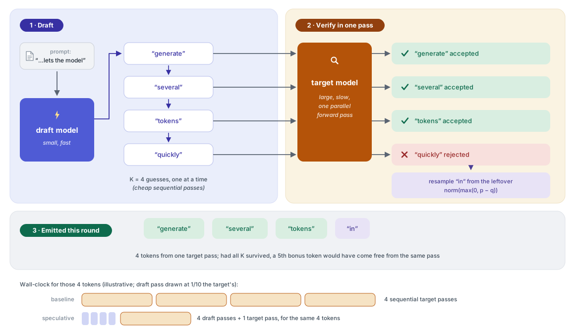
Notice the worst case: the very first draft token is rejected. Even then the round emits one token (the resampled one), so a round never produces less than plain decoding; it only wasted the cheap draft work. The best case emits \(K+1\) tokens for a single target pass. Every accepted guess is a target-model forward pass that never had to happen.
The obvious objection is the one worth dwelling on: if a small model’s guesses were reliable, why run the big model at all? The answer is that language is a mix of hard and easy predictions. Continuations like closing brackets, common collocations, the second half of a word, boilerplate code, or a phrase copied from the prompt are nearly deterministic, and a tiny model nails them; the big model earns its keep on the genuinely uncertain tokens. Speculative decoding automatically routes the easy tokens to cheap hardware-time and the hard ones to expensive hardware-time, without anyone having to define “easy”. The acceptance rate is the definition, computed on the fly.
The rule that makes it exact
The claim that deserves suspicion is exactness: the emitted tokens are distributed identically to sampling from the target model alone, not approximately.2 This section proves it, because the proof is short and it is the intellectual heart of the method.
Fix one position, write \(p(x)\) for the target’s distribution and \(q(x)\) for the draft’s. The draft proposes \(x \sim q\), and we accept with probability \(\min(1, p(x)/q(x))\), a variant of rejection sampling, the classical statistical technique for converting samples from one distribution into samples from another. Intuitively: wherever the draft under-bets relative to the target (\(q(x) \le p(x)\)), its proposals are always kept; wherever it over-bets (\(q(x) > p(x)\)), proposals are kept only a fraction \(p(x)/q(x)\) of the time, trimming the excess.
Two quantities fall out immediately (both proved as tool 1 in the appendix). The total probability that a proposal is accepted is the overlap between the two distributions,
\[\alpha \;=\; \sum_x q(x) \min\!\left(1, \frac{p(x)}{q(x)}\right) \;=\; \sum_x \min(p(x), q(x)),\]and the probability mass that acceptance fails to deliver, \(p(x) - \min(p(x), q(x)) = \max(0, p(x) - q(x))\), sums to exactly \(1 - \alpha\). So on rejection (probability \(1-\alpha\)) we sample from that leftover mass, renormalized:
\[p'(x) \;=\; \frac{\max(0,\, p(x) - q(x))}{1 - \alpha}.\]Now the whole proof is one line. The probability that this position emits token \(x\) is
\[\underbrace{q(x)\min\!\left(1, \tfrac{p(x)}{q(x)}\right)}_{\text{proposed and accepted}} \;+\; \underbrace{(1-\alpha)\, p'(x)}_{\text{rejected, then resampled}} \;=\; \min(p(x), q(x)) + \max(0,\, p(x)-q(x)) \;=\; p(x).\]The two mechanisms are jigsaw pieces: acceptance delivers the part of \(p\) the draft covers, the residual delivers precisely the part it misses, and they sum to the target distribution exactly. No approximation, no tuning, any draft. A terrible draft costs speed (everything gets rejected), never correctness.
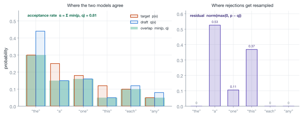
Three remarks worth internalizing:
- Greedy decoding is the easy special case. At temperature 0 the target “distribution” puts all mass on its argmax, and the rule degenerates to: accept the draft token if it equals the target’s argmax, else emit the argmax. That is Stern et al.’s 2018 scheme, recovered as a corollary.
- The rule is applied per position, left to right. Once token \(i\) is rejected, the later draft tokens are conditioned on a prefix that no longer exists, so they are useless and discarded. This is why the accepted tokens always form a prefix.
- Temperature and top-p fold in cleanly. The guarantee is about whatever distributions you hand the rule, so warping logits (temperature, top-k, top-p) before computing \(p\) and \(q\) preserves exactness with respect to the warped target, which is what “sampling from the model” means in production anyway.
How much faster: the arithmetic of acceptance
Speed now reduces to one question: how many tokens does a round emit? Model acceptance as an independent coin flip with probability \(\alpha\) per position, the simplification Leviathan et al. use for this calculation.3 A round emits \(i\) accepted tokens plus one more (the resample or the bonus), and the count is capped at \(K+1\), so the expected number of emitted tokens per target pass is a truncated geometric sum (tool 2 does the algebra):
\[\mathbb{E}[\text{tokens per round}] \;=\; \frac{1 - \alpha^{K+1}}{1 - \alpha}.\]At \(\alpha = 0.8\) and \(K = 4\) that is \((1 - 0.8^5)/0.2 = 3.36\) tokens per target pass, a 3.36x cut in target-model passes. Wall-clock speedup is lower because the draft is not free: with a draft pass costing a fraction \(c\) of a target pass, one round takes \(Kc + 1\) target-pass-equivalents, giving
\[\text{speedup} \;=\; \frac{1 - \alpha^{K+1}}{(1 - \alpha)(Kc + 1)},\]which at \(c = 0.05\) turns the 3.36 into \(3.36 / 1.2 = 2.80\)x. That is the shape of the numbers real deployments report.
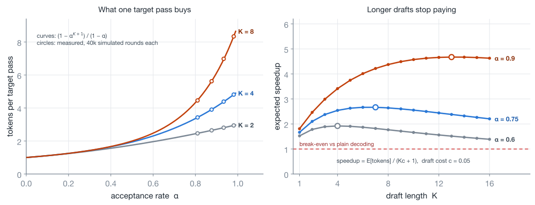
The left panel says drafts are nearly worthless below \(\alpha \approx 0.4\) (the curves pancake onto each other near 1-1.5 tokens per pass) and compound dramatically above 0.8. The right panel carries the operational lesson: the optimal draft length is finite and moves with acceptance. At \(\alpha = 0.6\), speedup peaks around \(K = 4\) and then declines, because each extra guess is increasingly likely to die in verification while still costing draft time. At \(\alpha = 0.9\) the optimum stretches to roughly \(K = 13\) at about 4.7x. This is why serving frameworks expose speculation length as a tunable and why some adapt it on the fly.
Checking the math honestly
Formulas about randomized algorithms are easy to misquote, so the numbers above are backed by a simulation you can run (the foldable block below): a 6-token vocabulary, a fixed target \(p\) and draft \(q\) with overlap \(\alpha = 0.810\), and 200,000 simulated rounds at \(K = 4\). Two checks:
- Exactness. The empirical distribution of all emitted tokens comes out to \((0.3003, 0.2502, 0.1791, 0.1203, 0.1002, 0.0499)\) against a target of \((0.30, 0.25, 0.18, 0.12, 0.10, 0.05)\): a maximum deviation of 0.0009, pure sampling noise. The accept/trim/resample plumbing really does reconstruct \(p\).
- Throughput. Measured tokens per round: 3.425. The formula predicts \((1 - 0.81^5)/0.19 = 3.428\). The circles in the left panel above repeat this check across twelve \((\alpha, K)\) combinations.
The speculative sampling simulation (click to expand)
Numpy only. spec_round is the algorithm exactly as described: sequential accept/reject down the draft, residual resample at the first failure, bonus token if everything survives. Positions are i.i.d. here (the same p and q at every step), which is the regime where the closed-form formula is exact.
import numpy as np


def residual(p, q):
    """The leftover distribution norm(max(0, p - q)) used after a rejection."""
    r = np.maximum(p - q, 0.0)
    return r / r.sum()


def spec_round(p, q, K, rng):
    """One speculative round: draft samples K tokens from q, the target
    accepts each with prob min(1, p/q); on the first rejection it resamples
    from the residual, and if all K survive it samples a free bonus token
    from p. Returns the emitted tokens (i.i.d. positions, so p and q are
    the same at every step)."""
    out = []
    for _ in range(K):
        x = rng.choice(len(q), p=q)
        if rng.random() < min(1.0, p[x] / q[x]):
            out.append(x)                                # accepted draft token
        else:
            out.append(rng.choice(len(p), p=residual(p, q)))
            return out                                   # correction, stop
    out.append(rng.choice(len(p), p=p))                  # all K survived: bonus
    return out


def run_rounds(p, q, K, n_rounds, seed):
    """Simulate n_rounds speculative rounds; return the empirical distribution
    of emitted tokens and the mean number of tokens emitted per round."""
    rng = np.random.default_rng(seed)
    counts = np.zeros(len(p))
    total = 0
    for _ in range(n_rounds):
        toks = spec_round(p, q, K, rng)
        total += len(toks)
        for t in toks:
            counts[t] += 1
    return counts / counts.sum(), total / n_rounds


def expected_tokens(alpha, K):
    """Leviathan et al. Eq. 1: E[tokens per round] for acceptance rate alpha."""
    return (1 - alpha ** (K + 1)) / (1 - alpha)


P = np.array([0.30, 0.25, 0.18, 0.12, 0.10, 0.05])       # target p
Q = np.array([0.44, 0.15, 0.16, 0.05, 0.12, 0.08])       # draft q
ALPHA = float(np.minimum(P, Q).sum())

print(f"alpha = {ALPHA:.3f}")
emp, mean_tok = run_rounds(P, Q, K=4, n_rounds=200_000, seed=1)
print("target p   :", np.round(P, 4))
print("empirical  :", np.round(emp, 4))
print(f"max abs dev: {float(np.abs(emp - P).max()):.4f}")
print(f"tokens/round measured {mean_tok:.3f} vs formula "
      f"{expected_tokens(ALPHA, 4):.3f}")

# alpha = 0.810
# target p   : [0.3  0.25 0.18 0.12 0.1  0.05]
# empirical  : [0.3003 0.2502 0.1791 0.1203 0.1002 0.0499]
# max abs dev: 0.0009
# tokens/round measured 3.425 vs formula 3.428
Implementing it against a real model
Against an actual transformer, the loop adds only two moving parts to the simulation above: the distributions come from model forward passes, and both models keep KV caches that must be rolled back when guesses die. In PyTorch-flavored pseudocode:
@torch.no_grad()
def speculative_step(target, draft, ids, K):
    """One round. Returns ids extended by 1..K+1 accepted tokens."""
    # 1) draft: K cheap autoregressive steps
    draft_ids = ids
    q = []                                   # draft dists, one per position
    for _ in range(K):
        q_t = softmax(draft(draft_ids).logits[:, -1])
        q.append(q_t)
        draft_ids = cat(draft_ids, sample(q_t))
    guesses = draft_ids[:, ids.shape[1]:]    # the K proposed tokens

    # 2) verify: ONE target pass over prefix + all K guesses
    #    logits at position i give the target's dist for token i+1,
    #    so one pass yields p_1 .. p_{K+1}
    p = softmax(target(draft_ids).logits[:, ids.shape[1] - 1:])

    # 3) accept / fix
    for i in range(K):
        x = guesses[:, i]
        if rand() < min(1.0, p[i][x] / q[i][x]):
            ids = cat(ids, x)                # accepted
        else:
            ids = cat(ids, sample(norm(clamp(p[i] - q[i], min=0))))
            rollback_kv_caches(target, draft, to_len=ids.shape[1])
            return ids                       # first rejection ends the round
    return cat(ids, sample(p[K]))            # all survived: bonus token
The structure to notice: the draft loop is the old sequential bottleneck, but run on a model small enough not to matter; the target appears exactly once per round, in a pass whose length-\(K{+}1\) input makes it barely more expensive than a length-1 decode step, per the roofline argument.
If you just want to use it, it is a flag, not a project. Hugging Face Transformers calls it assisted generation: model.generate(**inputs, assistant_model=small_model). vLLM takes a speculative_config specifying the method (draft model, EAGLE, or n-gram) and num_speculative_tokens; llama.cpp has --model-draft. The real implementation gotchas live at the systems level:
- Vocabulary agreement. The accept ratio \(p(x)/q(x)\) requires both models to speak the same token IDs, so target and draft must share a tokenizer. This, more than quality, is what limits off-the-shelf draft pairings.4
- Cache rollback. After a rejection, both models’ KV caches contain entries for tokens that officially never happened; forget to truncate them and generation silently corrupts.
- Batch shape churn. Different sequences in a batch accept different numbers of tokens per round, which is awkward for kernels and schedulers that like uniform shapes. This is a solved-but-annoying problem in production engines and part of why speculative decoding interacts poorly with very large batches (next section).
What actually moves the numbers
The formula says everything is downstream of two knobs: the acceptance rate \(\alpha\) and the draft cost \(c\). Real deployments add a third, batch size, that the formula silently assumed away.
The draft should be a scale model of the target, and there is an interior optimum. Acceptance is highest when the draft was trained on similar data with the same recipe, which is why families ship matched pairs (a 1B sibling drafting for a 70B). NVIDIA’s TensorRT-LLM measurements on Llama 3.1 405B make the tradeoff concrete: against a baseline of 33.5 tokens/s, a 1B draft reached 111.3 tokens/s (3.33x), a 3B draft 120.8 (3.61x), and an 8B draft 101.9 (3.04x). The 8B guesses better but costs too much per guess; the 1B is cheap but dies in verification more; the 3B wins. Knowledge distillation from the target is the standard way to push a small draft’s acceptance higher without paying for a bigger one.
Speculation length should track acceptance. The right panel of the speedup figure is the theory; practice agrees. Production guides treat \(\alpha \gtrsim 0.6\) with \(K\) around 3-5 as the healthy regime, stretching to 7-10 when acceptance is high (IBM’s PyTorch-blog work found code models tolerate roughly twice the speculation depth of prose, because code is more predictable). Google’s production setup drafts about 8 tokens ahead and lands 5-6 of them,5 and Hugging Face’s implementation adjusts the draft length on the fly: a few more guesses after a fully-accepted round, one fewer after a rejection.
Batch size is the boundary of the whole trick. Speculative decoding spends spare FLOPs, and continuous batching is the other consumer of the same slack: pile enough concurrent requests onto a GPU and decode’s matrix multiplies go compute-bound (measurements on A100 put the crossover around batch 32 for the weight matmuls6), at which point verification stops being free and speculation competes with throughput instead of buying latency. This is why vLLM’s own documentation rates speculative methods “high gain” at low request rates and only “medium” at high ones, and why it shines brightest in latency-sensitive, small-batch settings: chat, agents, code assistants, local inference.
And when the stars align, it is spectacular. The draft’s dream scenario is text whose continuation is nearly deterministic given the context: editing code that already exists in the prompt, quoting from a retrieved document, filling boilerplate. Acceptance soars and the big model glides through entire spans at draft speed.
Where the draft comes from now
Everything so far assumed the draft is a separate small LM, which is where the field started but not where it settled. Maintaining a second model is operationally annoying (two artifacts to deploy, memory for both, a tokenizer constraint), so the last two years have largely been about getting the draft from somewhere else.
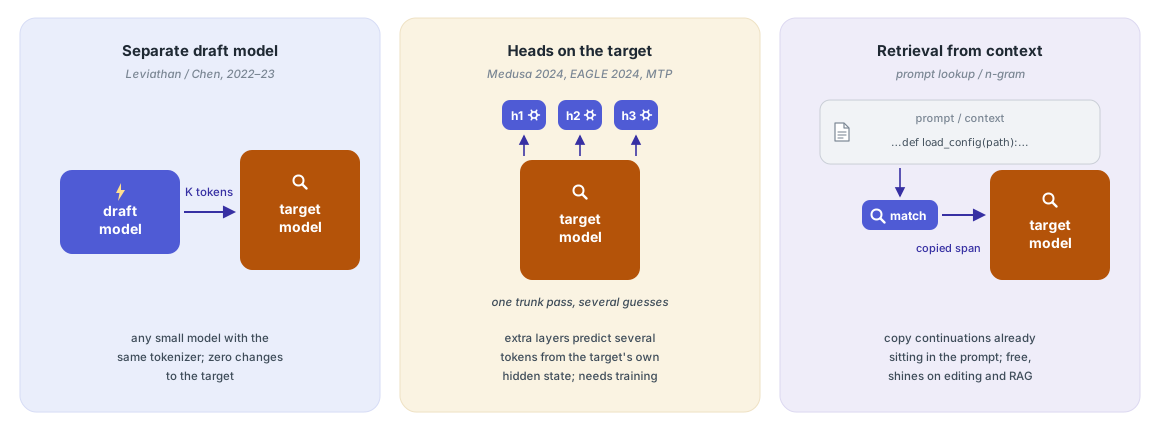
Heads on the target. Medusa (2024) returned to Stern et al.’s original architecture with modern machinery: bolt several extra output heads onto the target so one trunk pass yields guesses for the next few positions, assemble the candidates into a tree, and verify the whole tree at once using a crafted attention mask (“tree attention”), for 2.2-3.6x speedups. One honesty caveat: Medusa’s typical acceptance scheme keeps tokens the target merely rates as plausible rather than running exact rejection sampling, so at nonzero temperature its output distribution is close to, but not identical to, the target’s.7 The EAGLE line fixed that while going faster: its one-layer head autoregresses in the target’s feature space (next-hidden-state prediction, which is more regular than next-token prediction) and keeps the exact acceptance rule, with EAGLE-2 sizing the guess tree dynamically by draft confidence and EAGLE-3 reaching up to 6.5x in the best cases while holding a throughput edge even at batch 64. The same idea has migrated into pre-training itself: models like DeepSeek-V3 train multi-token prediction heads from the start, getting a built-in draft “for free” as a side effect of a training objective.
No model at all. Prompt lookup decoding replaces the draft with string matching: if the last few generated tokens also occur earlier in the context, propose the tokens that followed them there. It is free, needs nothing trained, and gets ~2.4x on summarization and document QA, where outputs quote inputs constantly; it ships in vLLM as the ngram method and in Transformers as prompt_lookup_num_tokens. Lookahead decoding goes further and has the target generate its own guesses via Jacobi-style parallel iteration, burning enormous extra FLOPs per step, which is viable for exactly the reason this post opened with: at batch 1 those FLOPs were idle anyway.
The through-line: speculative decoding is really a verification protocol, not a two-model architecture. The accept/reject rule does not care where guesses come from, so the industry keeps swapping ever-cheaper guess generators into the same exactness-preserving frame.
Two models, one voice
Step back and the design is worth admiring. Most inference optimizations buy speed with approximation: quantization perturbs the weights, cache eviction perturbs attention, distillation deploys a different model outright. Speculative decoding sits in the rare class that changes nothing about the output, joining the KV cache itself: the tokens that stream out are, in distribution, exactly the big model’s voice, even though a smaller model did most of the talking. The price is paid entirely in a currency the decode phase had in surplus: idle arithmetic.
What to take away:
- The opportunity is hardware-shaped. Decode runs at ~1 FLOP per byte on machines built for ~150, so scoring \(K\) tokens costs the same as generating one. Any method that converts sequential generation into parallel verification cashes this in; speculative decoding is the simplest such conversion.
- The correctness is one identity. Accepted mass \(\min(p,q)\) plus resampled mass \(\max(0, p-q)\) equals \(p\), per token, provably. Everything else (draft choice, speculation length, trees, heads) is engineering on top of a two-line proof.
- The economics are two numbers. Acceptance rate and relative draft cost set the ceiling via \(\tfrac{1-\alpha^{K+1}}{(1-\alpha)(Kc+1)}\); 2-3x is the going rate in production, and the trick dissolves precisely when its premise (idle compute) does, at large batch.
Speculation started as a decades-old CPU trick, jumped to transformers in 2018, became exact in 2022, and now quietly writes a good fraction of the AI text you read. The GPU was always fast enough to check several answers at once. Someone just had to notice that checking is not the same as writing.
Appendix: the derivation toolbox
Tool 1: the overlap and the leftover
Claim. With acceptance probability \(\min(1, p(x)/q(x))\) for a proposal \(x \sim q\): (a) the total acceptance probability is \(\alpha = \sum_x \min(p(x), q(x))\), and (b) the unnormalized residual \(\max(0, p(x) - q(x))\) sums to \(1 - \alpha\), so dividing by \(1-\alpha\) makes it a probability distribution.
Proof. (a) Condition on the proposal:
\[\Pr[\text{accept}] = \sum_x q(x)\min\!\left(1, \frac{p(x)}{q(x)}\right) = \sum_x \min(q(x), p(x)) = \alpha,\]where the middle step multiplies \(q(x)\) into the min (both branches: \(q(x)\cdot 1 = q(x)\) and \(q(x)\cdot p(x)/q(x) = p(x)\)). (b) For any two reals, \(\max(0, p - q) = p - \min(p, q)\): if \(p \ge q\) both sides are \(p - q\), otherwise both are 0. Summing over the vocabulary,
\[\sum_x \max(0, p(x) - q(x)) = \sum_x p(x) - \sum_x \min(p(x), q(x)) = 1 - \alpha. \qquad \blacksquare\]Tool 2: the expected-tokens formula
Claim. If each draft token is accepted independently with probability \(\alpha\), a round with draft length \(K\) emits \(\frac{1 - \alpha^{K+1}}{1-\alpha}\) tokens in expectation.
Proof. Let \(N\) be the number of accepted draft tokens. The round emits \(N + 1\) tokens in every case: the resampled correction if \(N < K\), the bonus token if \(N = K\). For a nonnegative integer variable capped at \(K\), expectation can be summed by tail probabilities: \(\mathbb{E}[N] = \sum_{i=1}^{K} \Pr[N \ge i]\), and \(\Pr[N \ge i] = \alpha^i\) (the first \(i\) flips all succeed). So
\[\mathbb{E}[N+1] = 1 + \sum_{i=1}^{K} \alpha^i = \sum_{i=0}^{K} \alpha^i = \frac{1 - \alpha^{K+1}}{1 - \alpha},\]the last step being the finite geometric series (multiply \(\sum_{i=0}^{K}\alpha^i\) by \(1-\alpha\) and watch the telescope collapse to \(1 - \alpha^{K+1}\)). \(\blacksquare\)
Dividing by the round’s cost in target-pass units, \(Kc + 1\), gives the speedup formula used in the body.
Sources and further reading
- Fast Inference from Transformers via Speculative Decoding (Leviathan, Kalman, Matias, Google; arXiv Nov 2022, ICML 2023 oral) — the paper that named the method; source of the acceptance rule, the expected-tokens formula, and the 2-3x T5-XXL results.
- Accelerating Large Language Model Decoding with Speculative Sampling (Chen et al., DeepMind, Feb 2023) — the independent concurrent derivation; 2-2.5x on Chinchilla 70B with a 4B draft.
- Blockwise Parallel Decoding for Deep Autoregressive Models (Stern, Shazeer, Uszkoreit, NeurIPS 2018) — the greedy-only ancestor of the whole draft-then-verify family.
- Looking Back at Speculative Decoding (Google Research, 2024) — retrospective by the original authors; the speculative-execution framing, the memory-bandwidth argument, and the AI Overviews production confirmation.
- A Hitchhiker’s Guide to Speculative Decoding (IBM on the PyTorch blog, 2024) — practitioner’s view; the code-vs-prose speculation-depth observation and batch-size caveats.
- Speculative Decoding (Modular’s inference handbook) — a clean systems-level taxonomy of the variant landscape, from separate drafts to EAGLE-3 and adaptive schedulers.
- The Machine Learning Practitioner’s Guide to Speculative Decoding (MachineLearningMastery) — accessible walkthrough with the draft-selection heuristics quoted in the practice section.
- Medusa (Cai et al., 2024), EAGLE / EAGLE-3 (Li et al., 2024-2025), Lookahead Decoding (Fu et al., 2024), and prompt lookup decoding (Saxena) — the draft-source variants in the landscape figure.
- TensorRT-LLM Speculative Decoding (NVIDIA, 2024) — the Llama 405B draft-size sweep (1B/3B/8B) quoted in the practice section.
- vLLM speculative decoding docs and Assisted Generation (Hugging Face, 2023) — how to actually turn it on, and vLLM’s own guidance on where gains shrink.
- QServe (Lin et al., 2024) — the A100 profiling behind the batch-size-32 compute-bound crossover cited in the batching discussion.
Footnotes
-
312 TFLOPS divided by 2.039 TB/s (A100 80GB SXM) gives a ridge point of about 153 FLOPs/byte. The roofline mental model, plotting achievable throughput against arithmetic intensity, is covered in the scaling post. ↩
-
In deployed systems the guarantee holds up to floating-point numerics: Chen et al. state their scheme preserves the target distribution “within hardware numerics”, and vLLM describes its implementation as lossless up to the same caveat. The math itself is exact. ↩
-
In reality α varies by position (easy tokens cluster), so the formula is a first-order model rather than a theorem about real text; it is what the field quotes, and the simulation below shows it is accurate when its assumption holds. ↩
-
Cross-tokenizer speculative decoding exists as a research direction, but every mainstream deployment (HF assisted generation, vLLM draft models, TensorRT-LLM, llama.cpp) requires an exact vocabulary match between draft and target. ↩
-
Per Jeff Dean on the Latent Space podcast (February 2026): the draft “predicts about 8 tokens ahead,” typically “5 or 6” are kept, amortizing weight movement roughly fivefold. Podcast numbers, not a paper benchmark. ↩
-
From the QServe paper’s A100 profiling: decode-phase fully-connected layers become compute-bound at batch sizes around 32, while decode attention stays memory-bound throughout (it reads the per-request KV cache, which grows with the batch). ↩
-
Medusa-1 (frozen backbone, heads only) with greedy verification is lossless; the quality-neutrality of the relaxed scheme at temperature is an empirical claim in the paper, not a guarantee. EAGLE, by contrast, keeps the exact speculative-sampling rule and proves distribution preservation. ↩