
Table of Contents
- TL;DR
- The problem: every token pays for every parameter
- The idea, stated precisely
- Where the idea comes from
- Routing is the hard part
- The modern recipe: many small experts, one shared
- What do the experts actually learn?
- The systems bargain
- The state of play
- What to take away
- Sources and further reading
Two days ago, Moonshot AI released Kimi K3, a 2.8-trillion-parameter model that early rankings place at the top of every open-weight leaderboard. Yet when K3 processes a token, the overwhelming majority of those 2.8 trillion parameters sit idle: each token is routed to just 16 of the model’s 896 experts per layer. That trick, called mixture of experts (MoE), is why essentially every notable open model of the past two years (DeepSeek-V3, Qwen3, Llama 4, gpt-oss, GLM, the Kimi family) introduces itself with two numbers, total parameters and active parameters, and why the gap between them keeps widening. This post explains what a MoE layer actually is, where the idea came from (it predates the Transformer by 26 years), why routing tokens to experts is deceptively hard, and how the modern recipe emerged that today’s frontier open models all share.
TL;DR
- A MoE layer replaces the Transformer’s feed-forward block with \(N\) parallel “expert” blocks and a learned router that sends each token through only \(k\) of them: \(y = \sum_i G(x)_i\, E_i(x)\), where \(G(x)\) has at most \(k\) nonzero entries. Attention is untouched; only the feed-forward compute becomes conditional.
- This decouples what a model knows from what it spends. Stored capacity grows with \(N\); per-token compute grows with \(k\). Scaling laws reward parameters, so MoE buys parameters without paying for them on every token, which is why a 2.8T-parameter model can be served at tens-of-billions-scale cost.
- Routing is the hard part. Left alone, routers collapse: in the toy MoE trained below, one expert ends up with two thirds of all traffic and the loss lands 3.2x higher than the balanced run. The fixes evolved from noisy gating and auxiliary balancing losses (2017 to 2022) to DeepSeek-V3’s auxiliary-loss-free bias method (2024), which balances load without polluting the training gradient.
- The modern recipe is fine-grained and shared: hundreds of small experts instead of a handful of big ones, roughly eight routed per token, plus one always-on shared expert for common knowledge. Activation ratios fell from Mixtral’s 27.6% (2023) to DeepSeek-V3’s 5.5% to below 2% for Kimi K3, if its reported active-parameter range holds.
- The bargain has a price: every expert must sit in memory even though few run, so MoE wins at pre-training and high-throughput serving and loses on a single memory-constrained GPU. That asymmetry explains both why frontier labs converged on it and why small local models often stay dense.
The problem: every token pays for every parameter
A dense Transformer spends most of its parameters in the feed-forward networks (FFNs). With model width \(d\) and the standard 4x expansion, each block’s FFN holds two weight matrices of \(4d^2\) each, so \(8d^2\) parameters against roughly \(4d^2\) for the block’s attention projections: about two thirds of the block sits in the FFN.1 And unlike attention, whose cost varies with context, the FFN applies the same full matrix multiply to every single token. In a dense model, parameters used equals parameters stored, every token, every layer.
That would be fine if parameters were cheap to run, but the scaling-laws story pushes hard in the other direction: model quality improves smoothly and predictably as parameter count grows, so everyone wants more parameters. In a dense model, every parameter you add to get smarter also makes every future token more expensive to train and serve, forever. The natural question is whether a model can hold a huge number of parameters while using only the relevant ones for each input. That is conditional computation, and mixture of experts is its most successful form.
The idea, stated precisely
Since the mechanism is simple enough to define completely, it is worth doing so before adding any history or engineering.
Definition (sparse MoE layer). Fix \(N\) expert networks \(E_1, \dots, E_N\) (each an ordinary FFN mapping \(\mathbb{R}^d \to \mathbb{R}^d\), that is, taking and returning a \(d\)-dimensional vector) and a router producing one weight per expert, \(G(x) \in \mathbb{R}^N\), of which at most \(k\) are nonzero, with \(k\) far smaller than \(N\). For a token’s vector representation \(x \in \mathbb{R}^d\), the layer computes
\[y \;=\; \sum_{i=1}^{N} \textcolor{#2a78d6}{G(x)_i}\; \textcolor{#c2410c}{E_i(x)}.\]Experts with \(\textcolor{#2a78d6}{G(x)_i} = 0\) are never evaluated, so the layer’s compute is that of \(k\) experts, while its capacity is that of all \(N\).
The color convention here recurs through the post and its figures: blue marks the router and its decisions, orange marks the compute that actually runs, and purple (later) marks the always-on shared path. The simplest concrete router, and still the backbone of most designs, is a single learned matrix \(W_g \in \mathbb{R}^{d \times N}\) (so \(x \cdot W_g\) turns the token’s \(d\) numbers into \(N\) expert scores) followed by a softmax2 restricted to the top \(k\) scores:
\[\begin{aligned} s &= x \cdot W_g && \textcolor{#7b8794}{\small\text{one score per expert, from one matrix multiply}} \\[4pt] \mathcal{T} &= \operatorname{top-}k(s) && \textcolor{#7b8794}{\small\text{the indices of the } k \text{ largest scores}} \\[4pt] \textcolor{#2a78d6}{G(x)_i} &= \frac{e^{s_i}}{\sum_{j \in \mathcal{T}} e^{s_j}} \;\text{ for } i \in \mathcal{T}, \text{ else } 0 && \textcolor{#7b8794}{\small\text{softmax over the survivors only}} \end{aligned}\]Two consequences follow immediately from the definition, and they are the entire reason MoE exists.
First, capacity and compute decouple. Storage grows linearly in \(N\); per-token FLOPs (floating-point operations, the raw count of arithmetic a forward pass performs) grow linearly in \(k\). A model can multiply its parameter count by adding experts while holding the per-token bill nearly constant, which is exactly the deal the scaling laws want and dense models cannot offer. This is why MoE models are described by two numbers. Mixtral 8x7B, the model that made open MoE mainstream, stores 46.7B parameters in total (not 8x7B = 56B, because the eight copies exist only for the FFNs; attention and embeddings are shared) but activates just 12.9B per token: capacity in the 47B class at roughly 13B-class compute.
Second, the layer stays trainable. Because the surviving weights come from a softmax and multiply the expert outputs, gradients flow through the router’s scores for the chosen experts, so router and experts learn jointly by ordinary backpropagation. The discrete top-\(k\) choice itself has no gradient, and everything difficult about MoE training (the next two sections) descends from that one missing gradient.
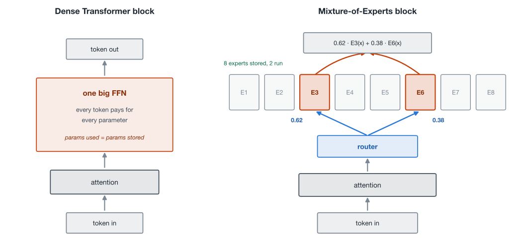
One clarification the “experts” name invites: nobody assigns the experts topics. The router and experts are trained end to end from random initialization, and whatever division of labor emerges is discovered, not designed. What actually emerges is stranger than the name suggests, and we will come back to it.
Where the idea comes from
1991: competing networks. Jacobs, Jordan, Nowlan and Hinton (1991) introduced adaptive mixtures of local experts: separate networks plus a softmax gate, trained on a multi-speaker vowel recognition task. Their lasting insight was about the loss function. Writing \(t\) for the target output the network should produce, \(o_i\) for expert \(i\)’s own prediction of it, and \(p_i\) for the gate’s weight on expert \(i\), the obvious choice of training error \(E\) compares the target against the gate-blended prediction:
\[E \;=\; \Big\lVert\, t - \sum_i p_i\, o_i \,\Big\rVert^2.\]This makes every expert compensate for the residual error of the whole blend, so all experts end up entangled in every case.3 Moving the sum outside the norm,
\[E \;=\; \sum_i p_i \,\lVert t - o_i \rVert^2,\]asks each expert to produce the entire answer on its own and lets the gate reward whichever one succeeds (each expert’s individual error is measured first, then blended by the gate weights). That single change turns cooperation into competition, and competition produces specialization. Every MoE since is a descendant of that observation.
2013: experts become a layer. For two decades the mixture was the whole model. Eigen, Ranzato and Sutskever (2013) reframed MoE as a stackable component: put one mixture layer after another, and a network with \(N\) experts per layer across \(L\) layers can express \(N^L\) expert combinations while storing only \(N \cdot L\) experts. On translated MNIST their first layer’s experts specialized by position and the second layer’s by digit class, an early glimpse of layers learning a factored division of labor. They also observed the gate collapsing onto favorite experts early in training and had to constrain it toward balanced usage: the first recorded sighting of the problem that would dominate the next decade.
2017: sparse and enormous. Shazeer et al. (2017), a Google Brain team including both Hinton and Jeff Dean, took the title of their paper seriously: “Outrageously Large Neural Networks.” They made the gate sparse (evaluate only the top \(k\) experts, not all of them) and scaled to models of up to 137B parameters and as many as 131,072 experts, sandwiched between LSTM layers, claiming over 1000x increases in capacity at minor compute cost. Their gate added tunable noise before the top-\(k\) cut,
\[H(x)_i = (x \cdot W_g)_i + \varepsilon_i \cdot \operatorname{Softplus}\big((x \cdot W_{\text{noise}})_i\big), \qquad \varepsilon_i \sim \mathcal{N}(0, 1),\]with \(G(x) = \operatorname{Softmax}(\operatorname{KeepTopK}(H(x), k))\). Here \(H(x)_i\) is expert \(i\)’s noisy score: the familiar routing score \((x \cdot W_g)_i\) plus standard Gaussian noise \(\varepsilon_i\), scaled by a second learned matrix \(W_{\text{noise}}\) that controls how much jitter each expert’s score receives.4 \(\operatorname{KeepTopK}\) then sets every non-surviving score to \(-\infty\) so the softmax zeroes it. The learned noise term jitters the ranking, so borderline experts occasionally win a token they would otherwise never see: exploration for a decision that has no gradient. The paper also introduced auxiliary losses penalizing imbalanced expert usage, ancestors of everything in the next section.
2020 to 2021: into the Transformer. GShard (Lepikhin et al., 2020) put sparse MoE inside a Transformer for the first time at scale, replacing every other FFN with a top-2 mixture in a 600B-parameter multilingual translation model trained across 2048 TPU chips. Then Switch Transformer (Fedus, Zoph and Shazeer, 2021) pushed the sparsity to its logical extreme: route each token to just one expert. Against the prevailing belief that \(k \geq 2\) was necessary for useful router gradients, top-1 worked, and the savings in router compute, communication, and per-expert batch size delivered the paper’s headline result: the same quality as a dense T5-Base up to 7x faster in pre-training wall-clock at equal FLOPs per token.5 Their Switch-C model reached 1.57 trillion parameters with 2048 experts back in 2021; the trillion-parameter era of the current open models is this lineage matured.
Routing is the hard part
Everything above makes MoE sound like a free lunch, so it is worth being precise about where the difficulty actually lives. The router makes a discrete choice per token, the choice has no gradient, and the system it controls is self-reinforcing: an expert that receives more tokens trains faster, gets better, earns higher router scores, and receives even more tokens. Left unregularized, this rich-get-richer loop collapses the mixture onto a handful of experts, and the idle majority become dead weight.
The classic countermeasure, standardized by Switch Transformer, is an auxiliary load-balancing loss added to the task loss. Over each training batch, let \(f_i\) be the fraction of the batch’s tokens actually routed to expert \(i\) (a hard count of routing decisions) and \(P_i\) the batch-average router probability assigned to expert \(i\) (soft and differentiable). The loss is
\[\mathcal{L}_{\text{aux}} \;=\; \alpha \, N \sum_{i=1}^{N} f_i \, P_i,\]with \(\alpha \approx 10^{-2}\). The design is cleverer than it looks. You cannot differentiate through the hard counts \(f_i\), so the loss pairs each count with its differentiable shadow \(P_i\): gradients flow through \(P\), pushing probability away from overused experts, while \(f\) supplies the ground truth about who is actually overused. The product is minimized exactly when routing is uniform (\(f_i = P_i = 1/N\)),6 and the factor \(N\) keeps \(\alpha\)’s meaning constant as expert counts change.
Watching the collapse happen
Routing collapse is easy to demonstrate honestly at toy scale. I trained a miniature Switch-style MoE with numpy: 8 linear experts and a linear top-1 router, on data drawn from 8 Gaussian clusters where each cluster has its own linear input-output rule. An ideal mixture assigns one expert per cluster. Both runs below are identical (same seed, same exploration noise on the router logits, annealed to zero) except that one adds the balancing loss above and one does not.
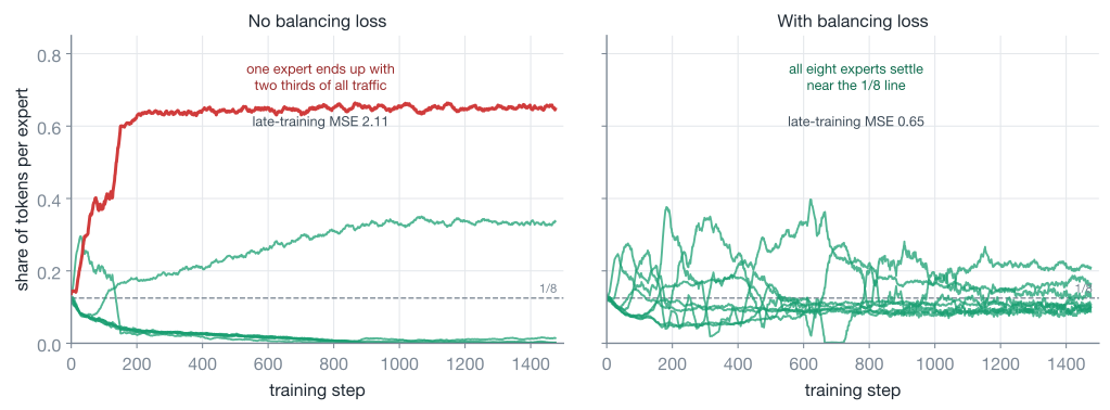
The unbalanced run is not subtly worse, it is qualitatively broken: one expert ends up serving five of the eight clusters with a single linear function, which no linear function can do. Traffic concentrates to a 65% / 33% split between two experts (the remaining six share the leftover 2%) and the mean squared error plateaus at 2.108. The balanced run holds every expert between a 9% and 21% share and reaches 0.654, a 3.2x improvement, because balance is what lets each expert own one cluster and fit it exactly.7 The full simulation, whose printed output is where every number in this paragraph comes from, is in the foldable block below.
The toy MoE simulation (click to expand)
Numpy only. The router and expert gradients are analytic (the same formulas a framework's autograd would produce for this model, with the hard counts treated as constants, as in Switch Transformer) and were verified against finite differences. Exploration noise on the routing logits anneals to zero over the first 60% of training in both runs.
import numpy as np


def moe_grads(W_r, W_e, x, y, aux_weight, n_exp, rng=None, noise=0.0):
    batch = x.shape[0]
    logits = x @ W_r.T
    z = np.exp(logits - logits.max(1, keepdims=True))
    p = z / z.sum(1, keepdims=True)                      # [batch, n_exp]
    route_logits = logits + (rng.normal(0, noise, logits.shape)
                             if noise else 0.0)
    top = route_logits.argmax(1)                         # top-1 routing
    onehot = np.eye(n_exp)[top]                          # [batch, n_exp]
    g = p[np.arange(batch), top]                         # gate value p_i
    e = np.einsum("bd,bd->b", W_e[top], x)               # expert output
    err = g * e - y
    mse = float(np.mean(err ** 2))
    share = onehot.mean(0)                               # f_i
    coef = (2.0 / batch) * err * g
    grad_W_e = (onehot * coef[:, None]).T @ x            # [n_exp, d]
    task_dlogit = (2.0 / batch) * (err * e * g)[:, None] * (onehot - p)
    aux_dlogit = (aux_weight * n_exp / batch) * p * (share[None, :]
                                                     - (p @ share)[:, None])
    grad_W_r = (task_dlogit + aux_dlogit).T @ x          # [n_exp, d]
    return mse, share, grad_W_r, grad_W_e


def simulate_moe(aux_weight, steps=1500, seed=0):
    rng = np.random.default_rng(seed)
    n_exp, d, batch, lr = 8, 2, 256, 0.05
    centers = rng.normal(0, 3, size=(n_exp, d))          # cluster centers
    true_w = rng.normal(0, 1, size=(n_exp, d))           # per-cluster linear fn
    W_r = rng.normal(0, 0.01, size=(n_exp, d))           # router
    W_e = rng.normal(0, 0.01, size=(n_exp, d))           # experts near zero
    share = np.zeros((steps, n_exp))
    mses = []
    for t in range(steps):
        c = rng.integers(0, n_exp, size=batch)           # which cluster
        x = centers[c] + rng.normal(0, 0.5, size=(batch, d))
        y = np.einsum("bd,bd->b", true_w[c], x)
        noise = 1.0 * max(0.0, 1 - t / (steps * 0.6))
        mse, share[t], gr, ge = moe_grads(W_r, W_e, x, y, aux_weight, n_exp,
                                          rng, noise)
        mses.append(mse)
        W_r -= lr * gr
        W_e -= lr * ge
    return share, float(np.mean(mses[-100:]))


for w in (0.0, 1.5):
    share, mse = simulate_moe(aux_weight=w)
    avg = share[-100:].mean(0)
    print(f"aux weight {w}: MSE {mse:.3f}, shares {np.round(avg, 2)}")

# aux weight 0.0: MSE 2.108, shares [0.   0.   0.01 0.   0.65 0.   0.   0.33]
# aux weight 1.5: MSE 0.654, shares [0.1  0.11 0.17 0.09 0.21 0.13 0.1  0.09]
The rest of the routing toolbox
Real systems layer several more mechanisms on top of the balancing loss, each solving a specific failure mode.
Expert capacity and token dropping. Accelerators want static tensor shapes, but routing is dynamic, so each expert is given a fixed budget of \((T / N) \times \text{capacity factor}\) tokens, where \(T\) is the number of tokens in the batch (GShard’s formulation; a capacity factor of 1.0 gives each expert exactly its fair share). Tokens that arrive at a full expert are dropped: they skip the FFN entirely and ride the residual connection (the skip path that adds a block’s input straight into its output) to the next layer unchanged. Switch showed that with decent balancing, capacity factors of 1.0 to 1.25 lose under 1% of tokens, an acceptable price for years, though the modern trend is to eliminate dropping altogether.
Numerical stability. The router’s softmax exponentiates its logits (the raw scores \(s\) before any normalization), which amplifies bfloat16 roundoff badly enough to destabilize very large runs; Switch cast just the router to float32, and ST-MoE (Zoph et al., 2022) added a router z-loss, \(c_z \cdot \text{mean}\big[(\log \sum_j e^{s_j})^2\big]\) with \(c_z = 10^{-3}\), which penalizes large logits before they ever reach the exponential.
Inverting the direction. Expert-choice routing (Zhou et al., 2022) flips the question: instead of each token picking its top experts, each expert picks its top tokens, filling a fixed bucket. Load balance then holds by construction, no auxiliary loss needed, and hard tokens can naturally receive more experts than easy ones. The catch is that choosing “the best tokens in the batch” means peeking across positions, which leaks future information in autoregressive decoding, so the idea fits encoders better than the decoder-only models that now dominate.
Balancing without a loss. The auxiliary loss works by injecting a gradient that fights the task gradient, and DeepSeek-V3 (2024) showed you can get the balance without the fight. Each expert carries a bias \(b_i\) that is added to its routing score only for the purpose of top-\(k\) selection; the gate value that actually multiplies the expert’s output still uses the raw score. After each training step, a controller nudges every \(b_i\) down if expert \(i\) ran over its fair share and up if it ran under, by a fixed step size \(\gamma\). Overloaded experts become slightly harder to select, underloaded ones easier, and the model’s learned preferences are never distorted by a balancing gradient because none exists.8 V3 trains this way with no token dropping at all, and reports that its experts show more genuine domain specialization than auxiliary-loss models, exactly the outcome the toy simulation’s footnote would predict: less interference, better experts.
The modern recipe: many small experts, one shared
If you compare Mixtral (2023) with DeepSeek-V3 (2024) or anything after it, the expert shape changed as much as the routing. The shift comes from DeepSeekMoE (Dai et al., 2024), which made two arguments about specialization.
Fine-grained segmentation. Slice each big expert into \(m\) small ones and route to \(m \cdot k\) of them, keeping parameters and FLOPs constant. What changes is combinatorics: with Mixtral’s 2-of-8 there are only \(\binom{8}{2} = 28\) possible expert teams per token, while DeepSeek-V3’s 8-of-256 offers \(\binom{256}{8} \approx 4.1 \times 10^{14}\). More possible teams means knowledge can be carved into finer, more composable pieces, instead of every expert being forced to be a generalist.
Shared-expert isolation. Some knowledge (basic syntax, common patterns) is needed by every token. If all experts are routed, each one must redundantly relearn that common core. DeepSeekMoE reserves one or more shared experts that every token passes through unconditionally, freeing the routed experts to store only what is genuinely specialized. Writing \(u\) for the token’s vector entering the MoE layer and \(h\) for the vector leaving it, a DeepSeek-V3 MoE layer computes
\[h \;=\; u \;+\; \textcolor{#5f4bb6}{\sum_{i=1}^{N_s} \mathrm{FFN}^{(s)}_i(u)} \;+\; \textcolor{#c2410c}{\sum_{i=1}^{N_r} \textcolor{#2a78d6}{g_{i}}\, \mathrm{FFN}^{(r)}_i(u)},\]with \(N_s = 1\) shared expert always on (purple, the third color of the convention; the superscripts \((s)\) and \((r)\) mark shared versus routed experts) and \(N_r = 256\) routed experts of which the top \(8\) receive nonzero gates \(\textcolor{#2a78d6}{g_i}\). The bare leading \(u\) is the residual connection carrying the token’s input forward. One more modern touch: V3 scores experts with a sigmoid per expert (each score squashed independently into a value between 0 and 1) rather than a softmax across experts, then normalizes over the chosen \(k\), so experts are judged on their own merits instead of competing in one big normalization.
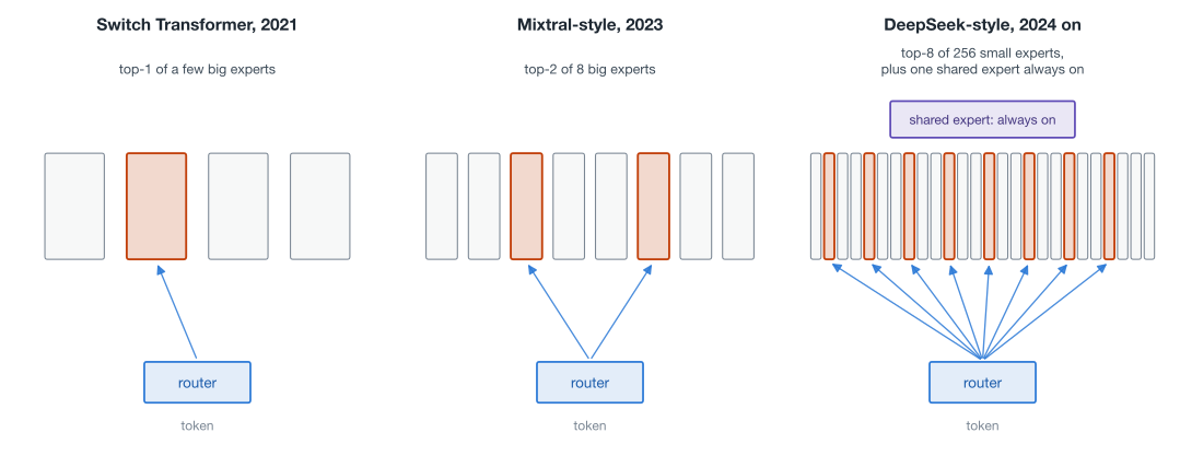
This recipe (fine-grained routed experts, a shared expert, top-8-ish selection, bias-based balancing) is, with local variations, what Kimi K2 (384 experts), Qwen3-Next (512 experts, 10 routed plus 1 shared active), and the rest of the current open cohort run on. The trend line inside the recipe is toward ever-sparser activation: Mixtral activated 27.6% of its parameters per token, DeepSeek-V3 5.5%, Kimi K2 3.2%, Qwen3-Next 3.8% of a much smaller total, and Kimi K3 lands under 2% if its reported active-parameter range holds.
What do the experts actually learn?
Given the name, you might expect a chemistry expert and a French expert. What large-scale inspection actually finds is stranger. The ST-MoE authors looked at what encoder experts specialize in and found shallow, token-level structure: an expert for punctuation, one for verbs, one for numbers, one for proper nouns. Decoder experts specialized far less. And in multilingual models, no expert became a language specialist: load balancing actively prevents it, because a dedicated French expert would be idle on every non-French batch, which is exactly the imbalance the balancing machinery is built to destroy. The experts are best thought of not as subject-matter specialists but as a learned, very wide vocabulary of feed-forward transformations that the router composes token by token.
That picture is starting to shift with the modern recipe: DeepSeek-V3 reports that dropping the auxiliary loss in favor of bias-based balancing produces visibly more domain-clustered expert usage. Softer balancing pressure seems to let more human-legible specialization survive, though “more than before” still falls well short of the tidy one-expert-per-topic story the name suggests.
The systems bargain
Everything MoE saves is compute; everything it costs is memory and plumbing. This asymmetry decides where it wins.
Memory scales with total parameters. Routing happens per token at runtime, so all \(N\) experts must be resident and ready. Mixtral needs the VRAM of a 47B model while computing like a 13B one; a K3-class model needs terabyte-scale weights resident (Moonshot ships it quantized to roughly 4 bits partly for this reason) regardless of how few parameters each token touches. For a home user with one GPU, the MoE deal can be actively bad: the dense 13B model that fits in memory beats the 47B MoE that does not. This is why the technique rules at datacenter scale and remains rarer at the small end.
At datacenter scale the plumbing is called expert parallelism. Different experts live on different chips, and each token is shipped to the chips holding its chosen experts and back again, an AllToAll communication pattern layered on top of the data, tensor, and pipeline parallelism that the scaling post walks through. Load balancing thus matters twice over: an overloaded expert is not just a modeling failure but a physical hot spot, one chip doing the work while its neighbors idle.
Training and fine-tuning carry their own quirks. Sparse models historically overfit small downstream tasks more readily than FLOP-matched dense models, and ST-MoE found they want the opposite fine-tuning protocol (smaller batches, higher learning rates), enough to erase the pre-training speedup if you get it wrong. Two later results softened the picture: instruction tuning turns out to benefit MoE models more than dense ones (Shen et al., 2023), and sparse upcycling (Komatsuzaki et al., 2022) showed you can warm-start an MoE by copying a trained dense model’s FFN into every expert and adding a fresh router, rather than paying for sparse training from scratch.
The state of play
The table below collects notable open-weight MoE models, from the release that started the open MoE era to this week’s. Every figure is from the linked paper, model card (usually its config.json), or official announcement in the sources section; “n/d” means the lab has not disclosed it.
| Model | Released | Total | Active | Routed experts | Routed per token | Shared |
|---|---|---|---|---|---|---|
| Mixtral 8x7B | Dec 2023 | 46.7B | 12.9B | 8 | 2 | no |
| DeepSeek-V2 | May 2024 | 236B | 21B | 160 | 6 | 2 |
| DeepSeek-V3 | Dec 2024 | 671B | 37B | 256 | 8 | 1 |
| Llama 4 Maverick | Apr 2025 | 400B | 17B | 128 | 1 | 1 |
| Qwen3-235B-A22B | Apr 2025 | 235B | 22B | 128 | 8 | no |
| Kimi K2 | Jul 2025 | 1T | 32B | 384 | 8 | 1 |
| gpt-oss-120b | Aug 2025 | 117B | 5.1B | 128 | 4 | no |
| Qwen3-Next-80B-A3B | Sep 2025 | 80B | 3B | 512 | 10 | 1 |
| Ling-1T | Oct 2025 | 1T | ~50B | n/d | n/d | n/d |
| Mistral Large 3 | Dec 2025 | 675B | 41B | n/d | n/d | n/d |
| GLM-5 / GLM-5.2 | Feb / Jun 2026 | 744B | 40B | 256 | 8 | 1 |
| Qwen3.5-397B-A17B | Feb 2026 | 397B | 17B | 512 | 10 | 1 |
| DeepSeek-V4-Pro | Apr 2026 | 1.6T | 49B | 384 | 6 | 1 |
| MiniMax-M3 | Jun 2026 | 428B | 23B | 128 | 4 | 1 |
| Nemotron 3 Ultra | Jun 2026 | 550B | 55B | 512 | 22 | 1 |
| Inkling | Jul 2026 | 975B | 41B | 256 | 6 | 2 |
| Kimi K3 | Jul 2026 | 2.8T | unconfirmed | 896 | 16 | n/d |
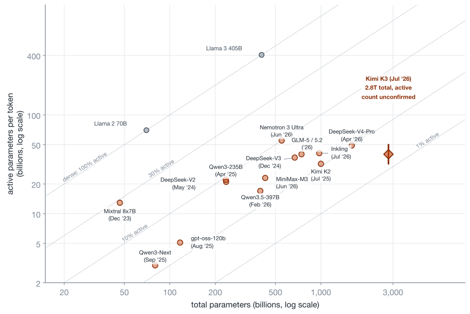
Read along the diagonals and the strategy of the era is legible at a glance: nobody is climbing the active-parameter axis. Active parameters have stayed between a few billion and a few tens of billions, the range that serves economically, while stored capacity has grown 60x. The scaling race moved into a direction where compute-per-token does not follow.
The 2026 wave shows the recipe is settled but not frozen. GLM-5.2 (744B total, 40B active, MIT license), whose training economics the distillation post dissects as a case study, took the top open-weights score on Artificial Analysis’ intelligence index with exactly the DeepSeek-shaped configuration of 256 routed experts, top-8, one shared. DeepSeek itself pushed to 1.6T total with V4-Pro while reducing routing to 6 experts per token, and Thinking Machines chose the same standard recipe for Inkling, its debut model: 975B total, 41B active, 256 routed plus two shared experts, trained multimodally from scratch. The interesting dissent comes from two directions: MiniMax-M3 swam against the fine-grained current with 128 larger experts at top-4, and NVIDIA’s Nemotron 3 Ultra routes 22 of 512 experts through a compressed latent space inside a hybrid Mamba-attention stack, evidence that the expert-shape question is not as closed as the rest of the recipe.
Kimi K3 is the current endpoint of the capacity line. Released on July 16, 2026 (API first, with weights promised by the end of July), it is the largest open-weight model ever announced: 2.8T total parameters, 896 experts of which 16 are routed per token, and, per Moonshot’s announcement, a 1M-token context built on a hybrid linear-attention design (“Kimi Delta Attention”, a continuation of the hybrid trend the attention post ends on) plus quantization-aware training that ships the weights at roughly 4 bits.9 Moonshot’s reported benchmarks and early third-party rankings place it above every other open-weight model and within reach of the strongest closed ones, with the usual caveat that cross-vendor agentic benchmarks run on different harnesses. For this post’s purposes the headline is simpler: the most capable open model in the world is a mixture of experts activating under 2% of itself per token, and nothing about that sentence would have been true of any frontier system three years ago.
The closed frontier is harder to see into, but not opaque. Google states outright that Gemini 1.5 was a sparse MoE, and OpenAI’s own open-weight gpt-oss models are MoE; GPT-4 was widely reported to be one as well, though that remains an unconfirmed leak.10 Whatever the specifics, the open record alone is enough for the conclusion: sparse expert models went from a Google research curiosity to the default architecture of frontier-scale language modeling in well under a decade.
What to take away
- MoE is one substitution with compounding consequences. Replace the FFN with routed experts and you decouple stored knowledge from per-token compute; every architectural detail since (noise, auxiliary losses, capacity factors, bias-based balancing, shared experts) is machinery for making that one substitution trainable and serveable.
- The interesting engineering is in the router, not the experts. The experts are ordinary FFNs. Thirty years of MoE progress, from Jacobs’ competitive loss to DeepSeek’s gradient-free balancing, is essentially the history of coaxing a non-differentiable decision into behaving inside a gradient-trained system, with a toy version of the failure reproducible in fifty-odd lines of numpy.
- Follow the two numbers. Total parameters tell you what a model can know and what it costs to hold; active parameters tell you what it costs to run. The entire open-frontier strategy of 2024 to 2026 is visible in that ratio falling from 28% to under 2%, and there is no sign the slide is finished.
Sources and further reading
- Mixture of Experts Explained (Sanseviero, Fedus et al., Hugging Face, 2023) — the survey this post’s practical sections lean on most; the source for the expert-capacity, fine-tuning, and specialization discussions.
- Adaptive Mixtures of Local Experts (Jacobs, Jordan, Nowlan, Hinton, 1991) — the origin; the competitive-versus-cooperative loss argument reproduced above.
- Learning Factored Representations in a Deep Mixture of Experts (Eigen, Ranzato, Sutskever, 2013) — MoE as a stackable layer.
- Outrageously Large Neural Networks (Shazeer et al., 2017) — sparse noisy top-k gating and the first 100B-scale mixtures.
- GShard (Lepikhin et al., 2020) and Switch Transformers (Fedus, Zoph, Shazeer, 2021) — MoE in the Transformer; expert capacity, top-1 routing, the auxiliary loss formulation used in the simulation, and the 7x speedup result.
- ST-MoE (Zoph et al., 2022) — router z-loss, fine-tuning protocols, and the expert-specialization inspections cited above; Expert Choice Routing (Zhou et al., 2022) for the inverted formulation.
- Mixtral of Experts (Jiang et al., 2024) — the 46.7B/12.9B numbers and the model that mainstreamed open MoE; Mixtral 8x22B announcement for the larger variant.
- DeepSeekMoE (Dai et al., 2024), DeepSeek-V2, and DeepSeek-V3 — fine-grained segmentation, shared experts, sigmoid gating, and auxiliary-loss-free balancing; the V2/V3 table rows.
- Model documentation for the 2023 to 2025 table rows: Llama 4, Qwen3, Kimi K2 and its model card, gpt-oss, Qwen3-Next-80B-A3B, Ling-1T, and Mistral Large 3.
- Model documentation for the 2026 table rows: GLM-5 and GLM-5.2 model cards (expert configuration from their
config.jsonfiles), Qwen3.5-397B-A17B, the DeepSeek-V4 release note and V4-Pro model card, MiniMax-M3, Nemotron 3 Ultra, Introducing Inkling (Thinking Machines Lab, 2026), and the Kimi K3 quickstart with early coverage by Simon Willison and MarkTechPost. - MoEs Meet Instruction Tuning (Shen et al., 2023) and Sparse Upcycling (Komatsuzaki et al., 2022) — the fine-tuning and warm-starting results.
- Gemini 1.5 technical report (Google, 2024) — the closed-frontier MoE confirmation.
Footnotes
-
The softmax turns any list of scores into positive weights summing to 1, by exponentiating each score and dividing by the total: \(\text{softmax}(s)_i = e^{s_i} / \sum_j e^{s_j}\). Larger scores get disproportionately larger weights, hence “soft max”: a differentiable approximation of picking the maximum. ↩
-
The double bars are the Euclidean norm: \(\lVert v \rVert^2\) is the sum of the squared entries of \(v\), so both versions of \(E\) are squared-error losses; they differ only in whether the blending happens before or after the error is measured. ↩
-
\(\operatorname{Softplus}(z) = \log(1 + e^z)\) is a smoothed ReLU that is always positive, so the learned noise scale can never go negative while staying differentiable. ↩
-
The 7x is Switch-Base versus T5-Base at fixed FLOPs per token and fixed data, measured as wall-clock time to reach T5-Base’s quality; the gain for the larger XXL configuration was 4x. Speedups of this kind depend on the baseline being FLOP-matched, not parameter-matched. ↩
-
Why uniform minimizes it: the router’s hard choices track its probabilities, so \(f_i \approx P_i\) and the sum behaves like \(\sum_i P_i^2\). By the Cauchy-Schwarz inequality \(\sum_i P_i^2 \geq (\sum_i P_i)^2 / N = 1/N\), with equality exactly when every \(P_i = 1/N\). ↩
-
Balance is not free either: sweeping the auxiliary weight in the same simulation gives MSE 0.558 at weight 0.5, 0.582 at 1.0, and 0.654 at 1.5, so pushing shares ever closer to uniform starts to cost accuracy. That interference between the balancing gradient and the task gradient is precisely the motivation for DeepSeek’s bias-based method described next. ↩
-
V3 keeps one tiny sequence-level balancing loss (the same \(f_i P_i\) shape, computed per sequence, with a very small coefficient) purely as a guard against pathological imbalance inside a single sequence. ↩
-
Moonshot had not published an official active-parameter count at the time of writing; secondary reports ranged from about 32B to about 50B (the latter being the naive 16/896 share of 2.8T). The figure, the shared-expert configuration, and the final license text all await the weight release and technical report. ↩
-
The GPT-4 claim (roughly 1.8T parameters across 16 experts, 2 routed per token) traces to 2023 reporting by SemiAnalysis and remarks by George Hotz, and was never confirmed or denied by OpenAI. Treat it as a rumor with decent provenance, not a fact. ↩