
In 1988 the roboticist Hans Moravec noticed something embarrassing about artificial intelligence: it is “comparatively easy to make computers exhibit adult level performance on intelligence tests or playing checkers, and difficult or impossible to give them the skills of a one-year-old when it comes to perception and mobility.”1 Nearly four decades later that paradox still defines robotics, but the way the field attacks it has been completely rebuilt, twice. This post traces that rebuild: how hand-engineered control gave way to reinforcement learning, why reinforcement learning then lost the manipulation battle to a much older idea (copying people), and how the last four years fused everything into robot foundation models that look strikingly like their language-model cousins. The goal is a self-contained tour: enough math to see why each transition happened, real numbers from the papers that drove it, and a running experiment you can reproduce.
Table of Contents
- TL;DR
- The problem, stated as a function
- The classical stack, and where it cracks
- Framing the robot as a learner
- The deep RL era: trial and error meets hardware
- The fork: simulation wins the legs
- Manipulation takes the other road: copying people
- The data gap and the foundation-model turn
- RL returns, wearing a post-training badge
- What’s still hard
- What to take away
- Appendix: the derivation toolbox
- Sources & further reading
TL;DR
- A robot’s controller is just a function from observations (pixels, joint angles) to actions (motor commands). Classical robotics builds that function by hand from four modules; every learning method in this post is a different way of fitting it from data instead.
- Reinforcement learning was the first serious challenger (roughly 2013 to 2019). It produced landmark demos (QT-Opt’s 580k real grasps, OpenAI’s cube-juggling hand) but real-world trial and error turned out to be brutally expensive: months of robot time per skill, human-supplied resets, and a reward function you must engineer per task.
- The field then forked. For locomotion, RL inside a physics simulator plus sim-to-real transfer won outright, and every modern legged robot now walks on an RL policy trained this way, some in under 20 minutes of wall-clock time. For manipulation, simulation couldn’t capture contact and clutter, so the field pivoted to imitation learning from human teleoperation.
- Naive imitation fails predictably: small errors push the robot into states no demonstration covered, where it errs worse, and the failure compounds quadratically with horizon. In the toy experiment below, 92% of behavior-cloned rollouts drive off the road while the fix (training on the learner’s own states) fails 0% of the time. Action chunking and generative policies (ACT, Diffusion Policy) are what made imitation practical without an interactive expert.
- The current era welds a web-pretrained vision-language model to a fast action generator: the vision-language-action model (RT-2, π0, Helix, GR00T). The recipe now mirrors LLMs exactly: pretrain on the internet, mid-train on pooled robot demonstrations, then post-train with RL so the robot can exceed its demonstrators, which is precisely where RL has re-entered the story.
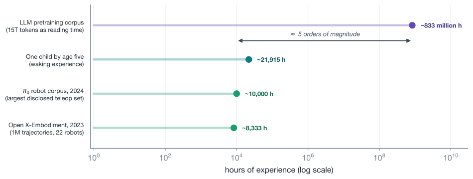
- The binding constraint is data. The largest disclosed robot datasets are around 10,000 hours of experience; an LLM’s text corpus, read aloud, is roughly 830 million hours. Most disagreements between serious robotics labs today are disagreements about how to close that five-order-of-magnitude gap.
The problem, stated as a function
Strip away the hardware and a robot controller is a function
\[a_t = \pi(o_t)\]that maps the current observation \(o_t\) (camera images, joint angles, gripper force) to an action \(a_t\) (target joint positions or torques for the next instant). Everything in this post, classical or learned, is a way of constructing a good \(\pi\). What makes robotics unusual among ML problems is a third axis beyond data and compute: the function has to run in real time, because the world does not pause while it thinks. A language model can ponder its next token for three seconds and nobody is harmed; a robot pouring coffee cannot.2 Typical low-level control loops run at 50 to 1000 Hz, which budgets a few milliseconds per decision and will matter a great deal when we get to modern architectures.
The classical stack, and where it cracks
For most of robotics history, \(\pi\) was assembled from four hand-built modules: perceive the scene, estimate the state of everything in it, plan a trajectory, and control the motors to track that plan.
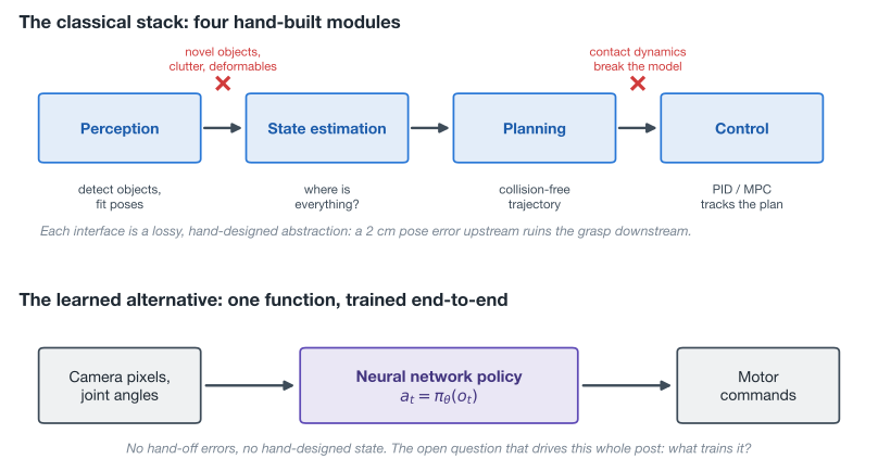
The classical stack is genuinely powerful where its assumptions hold. The robot’s own body obeys the manipulator equation
\[M(q)\ddot{q} + C(q,\dot{q})\dot{q} + g(q) = \tau,\]which says the torques \(\tau\) you apply must cover inertia (the mass matrix \(M\) times joint accelerations), velocity-dependent Coriolis effects \(C\), and gravity \(g\), all as known functions of the joint angles \(q\). Because the robot is built in a factory, \(M\), \(C\) and \(g\) are known almost exactly, so you can plan trajectories by optimization and track them with simple feedback like PID, or re-solve a short-horizon optimization at every tick, which is model predictive control (MPC). This is why Boston Dynamics-style locomotion worked years before learning did: a walking robot is essentially one well-modeled rigid body whose contact with the world happens at a few known points (its feet), so momentum can be regulated by carefully scheduled foot forces.3
The stack cracks in two places. First, perception: the pipeline assumes a state estimator can deliver “the mug is at (x, y, z) with pose R,” which works in a factory cell with known objects and fails in a home, because clutter, occlusion, novel objects and deformables (laundry, cables, food) have no compact hand-designable state at all. Second, contact: the moment a task involves rich contact, the clean dynamics above stop being the hard part. Contact is hybrid (modes switch discretely as surfaces touch and separate), frictional, and discontinuous, and optimizing trajectories through it is possible but brittle (Posa et al., 2014). Worse, in manipulation the dynamics that matter belong to the object, whose mass, friction and geometry the robot has never seen before. Each module’s errors also cascade: a 2 cm pose error upstream ruins the grasp downstream, and every new task needs its state representation, cost function and recovery logic re-engineered by hand.
Learning proposes to replace the whole chain with a single trained function. The question that organizes the next twenty years is simply: trained by what signal? The field’s three answers, in order, were reward, demonstrations, and the internet plus both.
Framing the robot as a learner
To learn \(\pi\) we need the problem in a form optimization can bite on, and the standard one is the Markov decision process: states \(s\), actions \(a\), transition dynamics \(P(s_{t+1} \mid s_t, a_t)\) that the world provides, and a reward \(r(s_t, a_t)\) that we must specify. A stochastic policy \(\pi_\theta(a \mid s)\) with parameters \(\theta\) is then scored by its expected discounted return,
\[J(\theta) = \mathbb{E}_{\tau \sim \pi_\theta}\!\left[\sum_{t=0}^{T} \gamma^{t}\, r(s_t, a_t)\right],\]where \(\tau\) is a trajectory rolled out under the policy and \(\gamma \in [0,1)\) trades off near against far rewards. We derived the gradient of this objective from scratch in the policy gradients post; the punchline, via the log-derivative trick, is
\[\nabla_\theta J(\theta) = \mathbb{E}_{\tau \sim \pi_\theta}\!\left[\sum_{t=0}^{T} \nabla_\theta \log \pi_\theta(a_t \mid s_t)\, R(\tau)\right],\]and the property that makes it beautiful for robotics is that the environment’s dynamics \(P\) dropped out entirely: you can improve a policy from sampled experience without ever modeling the physics. The estimator is noisy, so practical algorithms subtract a learned baseline and weight by advantages instead of raw returns, the construction we built step by step in the actor-critic post; PPO, the workhorse you will see all over robot learning, is that same actor-critic with updates clipped so no single step moves the policy too far from the one that gathered the data.4
On paper, this dissolves the classical stack’s problems: no hand-built perception, no contact models, just reward. The catch is the fine print. Model-free RL needs on the order of \(10^5\) to \(10^7\) trials, and a real robot runs in real time, breaks, and wears out. Episodes need resets (someone must put the objects back). The reward \(r(s,a)\) is computed from privileged state in a simulator, but on a real robot “did the task succeed?” is itself a perception problem you must engineer per task. And untrained policies explore by flailing, which is unsafe near objects and people. A candid retrospective from the Google robotics team (Ibarz et al., 2021) reads as a catalog of exactly these four taxes.5
The deep RL era: trial and error meets hardware
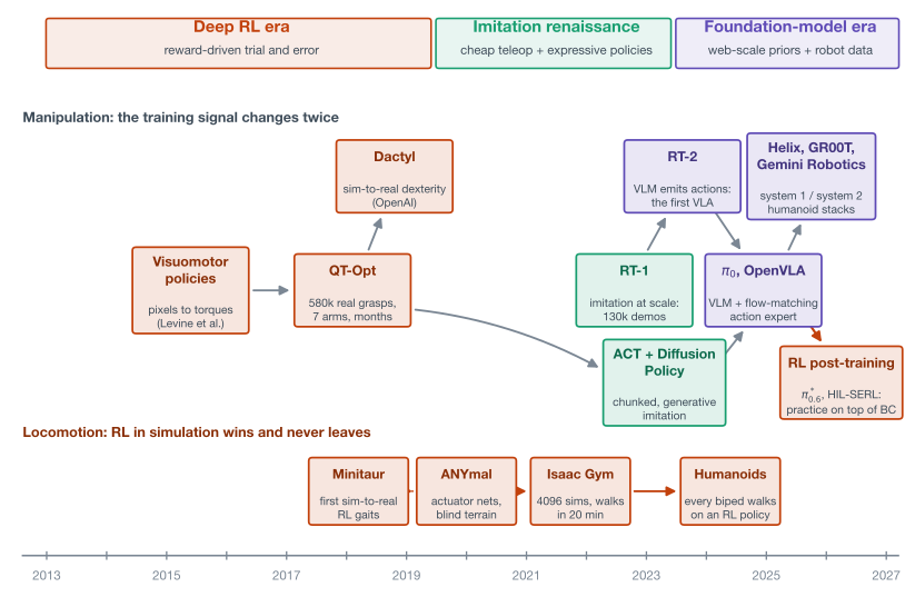
The era opens with Levine et al. (2016) training the first deep network to map raw camera pixels directly to motor torques on a real robot, screwing caps onto bottles with a 92,000-parameter CNN. The trick (guided policy search) was to let trajectory optimization solve each task instance locally, then distill the solutions into a vision-based network, which both proved the “pixels to torques” thesis and exposed its cost: instrumented training setups and one policy per task.
Scale was the obvious next move, and Google’s QT-Opt (Kalashnikov et al., 2018) is the era’s high-water mark: seven robot arms collecting about 580,000 real grasp attempts over months, feeding a distributed Q-learning system that reached 96% grasp success on unseen objects and displayed genuinely emergent closed-loop behavior like nudging clutter apart before grasping. It remains the strongest existence proof that real-world RL works at industrial scale, and simultaneously the strongest evidence against it: months of robot-farm time bought one skill whose reward (“is something in the gripper?”) happened to be automatable. Manipulation needs thousands of skills.
The alternative to paying reality’s data prices is simulation, where experience is cheap and reward functions can peek at privileged state. The problem is that policies overfit the simulator’s inevitably-wrong physics, and the era’s answer was domain randomization (Tobin et al., 2017 for visuals, Peng et al., 2018 for dynamics): don’t make the simulator accurate, make it varied. Train one policy across thousands of randomly perturbed worlds,
\[\max_\theta \; \mathbb{E}_{\xi \sim p(\xi)}\!\left[\, J_\xi(\theta) \,\right],\]where \(\xi\) bundles the randomized parameters (masses, friction, latencies, lighting), so that reality becomes just another sample from the training distribution. OpenAI’s Dactyl (2018) pushed this to its logical extreme: a 24-DoF hand reorienting a cube, trained with PPO on roughly a hundred years of simulated experience, transferring zero-shot to real hardware, with a recurrent policy that implicitly identifies the current world’s physics on the fly. The follow-up Rubik’s Cube system (2019) added automatic curriculum over the randomization ranges and still needed thousands of GPU-hours for one fragile skill. OpenAI disbanded its robotics team in 2021, citing insufficient data, and the field read that as the era’s closing verdict on brute-force RL for manipulation.6
The fork: simulation wins the legs
Here the story splits, because for locomotion the sim-to-real recipe simply worked, and understanding why illuminates everything that follows.
A legged robot is the one system where the simulator’s job is easy: the robot itself is known exactly from CAD, the world only touches it through a few brief foot contacts, and the reward (track a velocity command, stay upright, don’t waste energy) is computable from proprioception alone. The residual gap concentrates in the actuators, and ETH Zurich’s landmark ANYmal work (Hwangbo et al., 2019) closed it by training a small supervised network on real actuator data and embedding it inside the fast simulator, after which RL policies ran faster than the robot’s model-based controller and could get up from arbitrary falls. Lee et al. (2020) then produced blind quadrupeds crossing mud, snow and rubble by training a teacher with privileged terrain knowledge in sim and distilling it into a student that sees only its own proprioceptive history (the same student-mimics-teacher move as knowledge distillation, here crossing an information gap rather than a size gap), and the perceptive successor (Miki et al., 2022) took ANYmal up a 2.2 km Alpine hike with zero falls. The economics collapsed too: with GPU-native physics, Rudin et al. (2021) trained 4,096 simulated robots in parallel and produced deployable walking policies in under 20 minutes on a single GPU. That codebase became the template for the humanoid wave; essentially every biped you have seen walk in the last three years walks on an RL policy trained in randomized simulation.
Manipulation got no such gift, for reasons worth being precise about. Contact in manipulation is not a few clean foot strikes but sustained, multi-point, frictional interaction where simulators’ approximations are quantitatively wrong exactly where the task lives (insertions bind, grasps slip). The dominant dynamics belong to unknown objects rather than the known robot, deformables are both expensive to simulate and hard to even parameterize for randomization, and the policy must perceive object-level detail (texture, transparency, “the mug’s handle”) where photorealism gaps bite hardest. Domain randomization papers over low-dimensional gaps like friction and latency; it cannot cover “every object in a kitchen.” So while legs stayed with RL, hands went looking for a different training signal, and found the cheapest simulator of reality available: reality, with a human driving.
Manipulation takes the other road: copying people
Imitation learning is older than deep RL and looks almost insultingly simple. Collect demonstrations \(\mathcal{D} = \{(s_i, a_i)\}\) by teleoperating the robot, then fit the policy by maximum likelihood, exactly like supervised learning:
\[\theta^{*} = \arg\max_\theta \sum_{(s_i, a_i) \in \mathcal{D}} \log \pi_\theta(a_i \mid s_i),\]which for a Gaussian policy with fixed variance reduces to mean-squared error on actions. This is behavior cloning (BC), and it inherits none of RL’s taxes: no reward engineering, no exploration, no resets beyond what the human does anyway. Yet it was dismissed for two decades, for one theoretical reason and one practical one.
The theoretical reason is compounding error. Supervised learning guarantees small error on the training distribution, but a policy generates its own future inputs: one small mistake nudges the robot into a state the demonstrator never visited, where the policy errs worse, drifting further off-distribution in a vicious circle. Ross & Bagnell (2010) made this precise: if the cloned policy errs with probability at most \(\varepsilon\) per step on the expert’s states, its expected total cost over a horizon of \(T\) steps can exceed the expert’s by
\[J(\hat{\pi}) \;\le\; J(\pi^{*}) + \varepsilon\,\frac{T(T+1)}{2} \;=\; J(\pi^{*}) + O(\varepsilon T^{2}),\]quadratic in the horizon, versus the \(O(\varepsilon T)\) you’d naively expect, because an early mistake can poison every subsequent step. The proof is four lines and lives in tool 1 of the appendix. Rather than trust the bound, though, let’s watch it happen. I built a toy world (the full simulation is in the foldable block below, runnable with nothing but numpy): a point robot drives along a winding road, an expert steers it back toward the centerline, and a learner clones the expert from 20 clean demonstrations. At deployment we add ordinary actuation noise and watch what happens the moment the robot leaves the whisker-thin tube of states the demos covered.
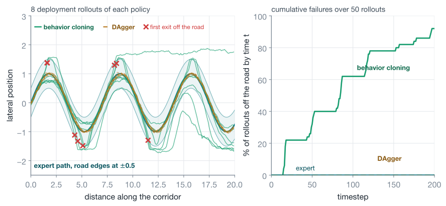
By step 200, 92% of behavior-cloned rollouts have left the road; the fix fails 0% of the time. The fix shown is DAgger (Ross et al., 2011), and it is four lines of code wrapped around the same supervised learner: roll out the learner’s policy, ask the expert to label the states it actually visited, aggregate, refit.
S_agg, a_agg = S_expert.copy(), a_expert.copy()
learner = fit(S_agg, a_agg)                      # plain behavior cloning
for _ in range(4):
    S_new = rollout(learner)                     # visit the learner's own states
    a_new = expert_labels(S_new)                 # ask the expert about *those*
    S_agg, a_agg = stack(S_agg, S_new), stack(a_agg, a_new)
    learner = fit(S_agg, a_agg)
# printed output (full runnable version in the foldable block below):
#   off the road by t=200:  BC 92%,  DAgger 0%,  expert 0%
Run the toy experiment yourself (self-contained, numpy only)
This is the exact simulation behind the figure and every number quoted above: same seed, same draw order, identical printed output. The expert steers toward a sine-wave centerline; the learner is ridge regression on narrow radial basis features, so it is only reliable near states it has seen.
import numpy as np

rng = np.random.default_rng(7)
A, W, DX, T, CLIP = 1.0, 0.9, 0.10, 200, 0.15

def path(x):
    return A * np.sin(W * x)

def expert(x, y):
    return float(np.clip(0.5 * (path(x + DX) - y), -CLIP, CLIP))

def rollout(policy, episodes, noise, spread):
    S, a, dev = [], [], []
    for _ in range(episodes):
        x, y = 0.0, rng.normal(0.0, spread)
        d = []
        for _ in range(T):
            u = policy(x, y)
            S.append((x, y))
            a.append(u)
            y = y + u + rng.normal(0, noise)
            x = x + DX
            d.append(abs(y - path(x)))
        dev.append(d)
    return np.array(S), np.array(a), np.array(dev)

# RBF ridge regression: a learner that is only reliable near seen states
cx, cy = np.linspace(0, T * DX, 24), np.linspace(-2, 2, 12)
CX, CY = np.meshgrid(cx, cy)
C = np.stack([CX.ravel(), CY.ravel()], axis=1)

def feats(S):
    S = np.atleast_2d(S)
    return np.exp(-0.5 * (((S[:, None, 0] - C[None, :, 0]) / 1.2) ** 2
                          + ((S[:, None, 1] - C[None, :, 1]) / 0.12) ** 2))

def fit(S, a):
    Phi = feats(S)
    w = np.linalg.solve(Phi.T @ Phi + 1e-3 * np.eye(Phi.shape[1]), Phi.T @ a)
    return lambda x, y: float(np.clip(feats([[x, y]])[0] @ w, -CLIP, CLIP))

S_exp, a_exp, _ = rollout(expert, 20, noise=0.004, spread=0.01)  # clean demos
bc = fit(S_exp, a_exp)                                # behavior cloning
_, _, dev_bc = rollout(bc, 50, 0.02, 0.05)            # noisy deployment
_, _, dev_ex = rollout(expert, 50, 0.02, 0.05)

learner, S_agg, a_agg = bc, S_exp, a_exp              # DAgger: 4 rounds
for _ in range(4):
    S_new, _, _ = rollout(learner, 10, 0.02, 0.05)    # learner's own states
    a_new = np.array([expert(x, y) for x, y in S_new])  # expert labels them
    S_agg, a_agg = np.vstack([S_agg, S_new]), np.concatenate([a_agg, a_new])
    learner = fit(S_agg, a_agg)
_, _, dev_da = rollout(learner, 50, 0.02, 0.05)

def off_road(dev):  # % of rollouts that ever exceed |deviation| = 0.5
    return 100 * np.maximum.accumulate(dev > 0.5, axis=1).mean(axis=0)[-1]

print(f"off the road by t={T}:  BC {off_road(dev_bc):.0f}%,"
      f"  DAgger {off_road(dev_da):.0f}%,  expert {off_road(dev_ex):.0f}%")
# -> off the road by t=200:  BC 92%,  DAgger 0%,  expert 0%
Training where you will be tested restores the honest \(O(\varepsilon T)\) bound. So why didn’t DAgger conquer robotics? That’s the practical reason BC stayed dismissed: DAgger needs an interactive expert on call to label arbitrary mid-failure states, which with human teleoperators roughly doubles the labor and is miserable to provide. What actually revived imitation, starting around 2022, was attacking the two failure modes architecturally instead:
- Action chunking. ALOHA/ACT (Zhao et al., 2023) built a \$20k bimanual teleop rig and trained a transformer to predict a chunk of the next ~100 actions at once instead of one action per tick. Fewer closed-loop decisions per episode means fewer chances for the state distribution to drift, directly shrinking the effective \(T\) in the bound above, and ACT hit 80-90% success on fine bimanual tasks (slotting a battery, opening a translucent cup) from around ten minutes of demonstrations per task.
- Generative action heads. Human demos are multimodal: you sometimes pass the obstacle on the left, sometimes on the right, and an MSE-trained policy averages the two into driving straight into it. Diffusion Policy (Chi et al., 2023) replaced the regression head with a conditional diffusion model over action chunks, so each sample commits to one coherent strategy, and reported an average 46.9% improvement over prior state of the art across 15 tasks.
Cheap rigs, chunking, and generative heads turned “collect a few hundred demos, train overnight” into a manipulation recipe that reliably worked, precisely the property RL never achieved on real hardware. The stage was set for someone to ask the obvious scaling question.
The data gap and the foundation-model turn
The scaling question has a number attached, and it is worth staring at. Llama 3 was pretrained on about 15 trillion tokens of text.7 Read aloud at a brisk 5 tokens per second, that corpus is \(15\times10^{12} / 5 / 3600 \approx 830\) million hours of human language experience. The largest disclosed robot-manipulation corpus used to train a single model, Physical Intelligence’s π0 pretraining set, is roughly 10,000 hours of teleoperation, and the pooled cross-institution Open X-Embodiment dataset holds a bit over one million trajectories, which at a generous 30 seconds each is about 8,300 hours. That is the field’s central fact: robot experience trails language experience by about five orders of magnitude, and unlike text, every new hour costs an hour of human labor, because the internet was never recording actions.8
The foundation-model era is a sequence of increasingly aggressive answers to that gap. RT-1 (Brohan et al., 2022) was imitation at scale: 130k demonstrations spanning 700+ tasks, collected by 13 robots over 17 months, absorbed by one transformer that hit 97% on seen tasks and generalized meaningfully better than per-task models. The pivotal move came with RT-2 (2023), which asked: why teach a robot model about the world from scratch when web-pretrained vision-language models already know what a mug is, what “extinct animal” means, and what kitchens look like? RT-2 co-fine-tuned a VLM to emit robot actions as text tokens alongside its usual web data, coining the term vision-language-action model (VLA), and the semantics transferred: roughly double RT-1’s success on unseen objects and scenes, and emergent instructions like “pick up the extinct animal” correctly fetching the toy dinosaur. Open X-Embodiment (2023) then showed the demonstrations themselves pool across bodies: a generalist trained on 22 different robots’ data outperformed each lab’s own specialist by about 50% on average, and open models followed (Octo, then the 7B OpenVLA (Kim et al., 2024), which beat the 55B RT-2-X by 16.5 points with 7x fewer parameters).
One engineering problem remained: an autoregressive VLM emitting discretized action tokens is slow and clumsy for dexterous, high-rate control. π0 (Black et al., 2024) supplied the now-dominant fix by welding a small action expert onto the VLM: the backbone digests images and language at its own leisurely pace, while a ~300M-parameter head trained with flow matching (the straightened-out descendant of diffusion) generates continuous 50-step action chunks, fast enough for 50 Hz control.
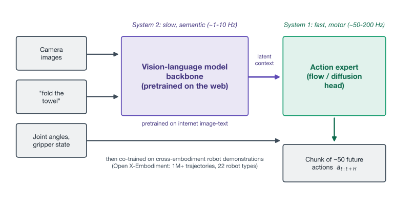
This “big slow understander, small fast mover” split is now everywhere, usually described in System 2 / System 1 language: Figure’s Helix runs a 7B VLM at 7-9 Hz feeding an 80M-parameter visuomotor policy at 200 Hz across a humanoid’s 35 upper-body degrees of freedom; NVIDIA’s GR00T N1 and Google DeepMind’s Gemini Robotics stack are architecturally the same idea. And the training pipeline has converged on a ladder any LLM engineer would recognize: pretrain the backbone on the web, mid-train the action expert on large cross-embodiment demo corpora, post-train on your robot and tasks, then adapt at deployment. π0.5 (2025) is the current landmark for what the recipe buys: mobile manipulators executing 10-15 minute cleaning tasks in homes they have never seen.
RL returns, wearing a post-training badge
Imitation has a ceiling built into its objective: a policy trained only on demonstrations can at best match its demonstrators, and it has never once seen its own mistakes, so it cannot learn to recover from them. It is learning to drive from videos of perfect driving.9 Breaking that ceiling requires learning from the robot’s own experience, which is RL’s home turf, and RL’s old taxes look very different when you start from a competent VLA instead of random flailing: exploration is mostly safe, failures are rare enough to label, and a value function has meaningful behavior to score.
Two 2024-25 results made this concrete. HIL-SERL (Luo et al., 2024) combined a handful of demos, off-policy RL, and live human corrections to reach near-100% success on precision tasks like timing-belt assembly within 1-2.5 hours of real-robot training, roughly doubling the success and speed of pure imitation. And Physical Intelligence’s π*0.6 with Recap (2025) scaled the idea to VLAs: train a value function over the robot’s rollouts, then condition the policy on a binarized advantage token (effectively “this was a good action” vs “a bad one”) and ask for “good” at deployment, folding demonstrations, teleoperated corrections, and autonomous practice into one recipe. The RL-tuned model roughly doubled throughput and more than halved failure rates on tasks like laundry folding, and ran an espresso bar all day. The analogy to language models is exact and explicitly drawn by the authors: pretraining gives knowledge, supervised fine-tuning gives competence, and RL on the model’s own outputs gives reliability, the same arc we traced for reasoning LLMs in the reasoning models post.10
So the 2026 division of labor reads: RL trained in simulation owns locomotion and whole-body control; imitation into VLAs owns manipulation’s foundation; and RL from real experience is the finishing school that pushes deployed skills toward the reliability that demos alone cannot reach.
What’s still hard
An honest close needs the other side of the ledger, because serious people disagree about how far along this all is.
- Data remains the war. The gap is five orders of magnitude, and the field’s three escape routes (fleet-scale teleoperation, simulation and world-model-generated synthetic data, and egocentric human video) all have credible champions and credible critics. Sergey Levine’s “Sporks of AGI” argues the surrogate routes smuggle in hand-designed assumptions that become the bottleneck (“the robot won’t master the real world unless it gets to see itself doing stuff in the real world”), while NVIDIA reports large gains from mixing synthetic data. Nobody knows the exchange rate yet.
- Evaluation barely scales. A policy’s success rate is measured by running a physical robot tens of times per condition, so published numbers are noisy, lab-specific, and largely incomparable; Ted Xiao’s prediction that “robot evaluation will become the biggest bottleneck of the 2020s” is aging well.
- Demos are not deployment. An 80% success rate makes a great video and a useless product; closing the reliability gap to “many nines” is exactly why the RL post-training turn matters, and it is far from done.
- Touch is missing. Rodney Brooks’s pointed critique observes that a human hand carries ~17,000 mechanoreceptors while today’s humanoid programs train on vision alone, with no touch-data tradition equivalent to the internet’s text and images; human-level dexterity may need a modality nobody is collecting at scale.
- Long horizons and memory. Minutes-long tasks work via subtask decomposition, but hour-scale autonomy with error recovery and persistent memory remains open; as Levine noted in late 2025, today’s VLAs typically act on about a second of context.
My own read after assembling this: the trend is real and the recipe (pretrain, imitate, then practice) is clearly the right shape, but the honest uncertainty is measured in “which decade,” and it lives almost entirely in the data and reliability bullets above.
What to take away
Three ideas organize forty years of this field. First, Moravec’s paradox is a data statement in disguise: evolution pretrained our sensorimotor systems for a billion years, the internet recorded our words but not our movements, and robotics is what machine learning looks like when the pretraining corpus is missing. Second, each era is defined by its training signal: hand-built models, then reward, then demonstrations, then the internet plus both, and each transition happened when the previous signal’s cost curve went vertical. Third, the frontier is a merger, not a winner: legs walk on simulated RL, hands imitate people, semantics come from the web, and reliability comes from practicing with reward, all in one stack. The robots are finally learning the way the rest of ML does, and what they are missing is not an algorithm but a childhood’s worth of experience.
Appendix: the derivation toolbox
1. Why cloning errors compound quadratically
Claim (Ross & Bagnell, 2010, who state it with the looser constant \(T^{2}\varepsilon\); the argument below keeps the sum exact). Consider a horizon of \(T\) decisions, per-step cost bounded in \([0,1]\), and a learned policy \(\hat{\pi}\) that, on the state distribution the expert visits at each step \(t\), disagrees with the expert \(\pi^{*}\) with probability at most \(\varepsilon\). Then
\[J(\hat{\pi}) \;\le\; J(\pi^{*}) + \varepsilon\,\frac{T(T+1)}{2},\]where \(J\) denotes expected total cost.
Proof. Run \(\hat{\pi}\) and couple it with the expert’s trajectory: as long as \(\hat{\pi}\) has made no mistake, it has chosen exactly the expert’s actions, so the state it occupies is distributed as an expert state. Let \(p_t\) be the probability that \(\hat{\pi}\) has made at least one mistake within the first \(t\) steps. At step \(t\), conditioned on no mistake so far, the state is expert-distributed, so a first mistake occurs now with probability at most \(\varepsilon\); by the union bound over steps,
\[p_t \;\le\; t\,\varepsilon.\]Now bound the cost at step \(t\). With probability \(1 - p_t\) the run is still mistake-free, so its expected cost is the expert’s cost at that step, call it \(c^{*}_t\). With probability \(p_t\) we know nothing and charge the worst case, cost 1. Hence the learner’s expected cost at step \(t\) is at most \((1-p_t)\,c^{*}_t + p_t \le c^{*}_t + p_t \le c^{*}_t + t\varepsilon\), using \(c^{*}_t \le 1\) in the middle step. Summing over \(t = 1, \dots, T\):
\[J(\hat{\pi}) \;\le\; \sum_{t=1}^{T} c^{*}_t + \varepsilon \sum_{t=1}^{T} t \;=\; J(\pi^{*}) + \varepsilon\,\frac{T(T+1)}{2}. \qquad \blacksquare\]The bound is tight in the worst case (an early mistake can be unrecoverable and cost 1 forever after, exactly like driving off the road), and the toy experiment in the body is a live instance: demonstrations cover a thin tube of states, one noisy step exits the tube, and the policy has no idea how to get back.
Why DAgger escapes it. DAgger trains on states drawn from the learner’s own rollouts, so its \(\varepsilon\) is measured on the same distribution it faces at test time, and the mistake-then-drift amplification never starts; there is no coupling argument to break. The formal guarantee, \(J(\hat{\pi}) \le J(\pi^{*}) + O(\varepsilon T)\) up to terms that vanish with enough iterations, is Theorem 3.2 of Ross, Gordon & Bagnell (2011) and rests on a reduction to no-regret online learning; the one-line intuition is simply train where you will be tested. The baseline-unbiasedness and advantage machinery used earlier in the post is proved step by step in the actor-critic post, so it is not repeated here.
Sources & further reading
Framing and field commentary
- Interlatent, “Modern AI Robotics from First Principles” — the reference that seeded this post; especially good on the real-time axis, edge vs cloud, and the training ladder.
- Sergey Levine, “Sporks of AGI” (2025) — the sharpest argument that surrogate data (sim, human video) cannot substitute for real robot experience.
- Ted Xiao, “What’s Missing for Robot Foundation Models?” (2025) — scaling laws, context, and the evaluation bottleneck, from inside Google DeepMind robotics.
- Rodney Brooks, “Why Today’s Humanoids Won’t Learn Dexterity” (2025) — the veteran skeptic’s case, centered on touch.
- Ibarz et al., “How to Train Your Robot with Deep RL: Lessons We’ve Learned” (2021) — candid retrospective on real-world RL’s four taxes.
- Google DeepMind, robotics lab tour with Hannah Fry (2025, video) — Hannah Fry visits DeepMind’s California robotics lab and probes Gemini Robotics-era robots on unseen objects; a rare unedited feel for what today’s generalization demos actually look like in person.
Deep RL era and sim-to-real
- Levine et al., end-to-end visuomotor policies (2016); Kalashnikov et al., QT-Opt (2018); OpenAI, Dactyl (2018) and Rubik’s Cube (2019).
- Tobin et al. (2017) and Peng et al. (2018) — visual and dynamics domain randomization.
- The locomotion streak: Hwangbo et al. (2019), Lee et al. (2020), Miki et al. (2022), Rudin et al. (2021), Kumar et al., RMA (2021).
Imitation renaissance
- Ross & Bagnell (2010) and Ross, Gordon & Bagnell, DAgger (2011) — the compounding-error theory.
- Zhao et al., ALOHA/ACT (2023); Chi et al., Diffusion Policy (2023); Chi et al., UMI (2024) — demonstrations without robots, via a hand-held gripper.
Foundation models and VLAs
- RT-1 (2022), RT-2 (2023), Open X-Embodiment (2023), OpenVLA (2024).
- π0 (2024), π0.5 (2025), π*0.6 / Recap (2025) — the Physical Intelligence line, and the clearest writeups of the pretrain/post-train recipe for robots.
- Figure, Helix (2025) and NVIDIA, GR00T N1 (2025) — System 1 / System 2 humanoid stacks; Gemini Robotics (2025).
- Luo et al., HIL-SERL (2024) — real-world RL made practical with human-in-the-loop corrections.
Textbook grounding
- Sutton & Barto, Reinforcement Learning: An Introduction — the RL fundamentals behind everything here, free online.
Footnotes
-
Hans Moravec, Mind Children (Harvard University Press, 1988). Steven Pinker later compressed the same observation into “the hard problems are easy and the easy problems are hard.” The usual explanation is evolutionary: perception and motor control encode roughly a billion years of optimization, while chess-style abstract reasoning is a recent, shallow layer. ↩
-
The coffee framing and the “robot as a function” lede are borrowed from Interlatent’s excellent first-principles tour of modern robot learning, which partly inspired this post. ↩
-
Boston Dynamics’ classical stack used reduced-order models, footstep planners, and whole-body MPC, with almost no machine learning through this era; they publicly described adopting RL for Spot’s locomotion controller only around 2023-24. ↩
-
The other staple is SAC, an off-policy actor-critic that maximizes reward plus policy entropy. Being off-policy it reuses old experience, making it far more sample-efficient, which is why it shows up whenever people train directly on real hardware. Both are sketched in the actor-critic post. ↩
-
Alex Irpan’s 2018 essay “Deep Reinforcement Learning Doesn’t Work Yet” is the classic candid assessment from inside the field, and it aged well. ↩
-
A parallel thread attacked sample cost with learned world models instead: train a dynamics model from experience, then train the policy inside its “imagination” (the Dreamer line). DayDreamer (Wu et al., 2022) got a real quadruped walking from scratch in about one hour this way, and world models are now resurfacing inside the data-generation strategies of the foundation-model era. ↩
-
The Llama 3 Herd of Models (Meta, 2024) reports the ~15T-token pretraining corpus. The 5 tokens/second reading rate is a deliberate back-of-envelope round number; the conversion is the one line of arithmetic shown in the text, and the conclusion is insensitive to it. ↩
-
UC Berkeley’s Ken Goldberg popularized this as the “100,000-year data gap”: 830 million hours of continuous reading is about 95,000 years, so the two framings agree. ↩
-
The driving-videos framing is again from the Interlatent post. The formal version is the compounding-error bound from earlier: demonstrations alone leave the \(O(\varepsilon T^2)\) term intact, and only training signal on the policy’s own states removes it, whether that signal comes from an interactive expert (DAgger) or from reward (RL). ↩
-
LLMs are also chipping at RL’s oldest tax from the other side: Eureka (Ma et al., 2023) had GPT-4 write and iteratively refine simulator reward functions, beating expert human-written rewards on 83% of 29 benchmark tasks. ↩