
Actor-Critic methods are a family of reinforcement learning algorithms that combine the benefits of value-based and policy-based approaches: an actor learns which actions to take, while a critic learns to judge how good those actions were and feeds that judgement back so the actor’s learning signal is far less noisy. This post builds the idea from the ground up: why pure policy gradients are noisy, how a baseline fixes that for free, and why the critic is really just a learned, state-dependent baseline.
Table of Contents
- TL;DR
- Background
- The Actor-Critic Approach
- Why Bother? The Variance Problem
- From REINFORCE to Actor-Critic in Four Steps
- Key Components
- The Algorithm Loop
- Variants of Actor-Critic Methods
- Applications
- Conclusion
- Further Resources
TL;DR
- An actor-critic pairs two learned functions: an actor \(\pi_\theta(a \vert s)\) that picks actions, and a critic \(V_w(s)\) that scores states.
- Pure policy-gradient methods like REINFORCE give unbiased but very noisy gradient estimates, which makes training slow and unstable.
- Subtracting a baseline from the reward leaves the expected gradient unchanged but shrinks its variance. In the toy problem below the reduction is exactly 5x.
- The critic is a learned, state-dependent baseline. Its one-step prediction error, the TD error \(\delta_t = r_{t+1} + \gamma V_w(s_{t+1}) - V_w(s_t)\), doubles as an estimate of how much better the chosen action was than average, and it is the feedback signal that updates both networks.
- The whole construction trades a little bias for a lot less variance, and it is the skeleton inside A2C, A3C, DDPG, TD3, SAC and PPO.
Background
Reinforcement Learning (RL) is a type of machine learning where an agent learns to make decisions by interacting with an environment: it observes a state, takes an action, receives a reward, and repeats, trying to maximise the reward it collects over time. RL methods can be broadly categorized into value-based and policy-based methods. In a previous post we walked through policy gradient algorithms along with a brief intro to RL, including a full derivation of the REINFORCE gradient estimator; we will lean on that result here, so it is worth a skim if policy gradients are new to you.
The Actor-Critic Approach
The core idea of Actor-Critic methods is to combine an “actor” (policy) and a “critic” (value function), where the actor’s job is to select actions given a state and the critic’s job is to critique the actions the actor takes.
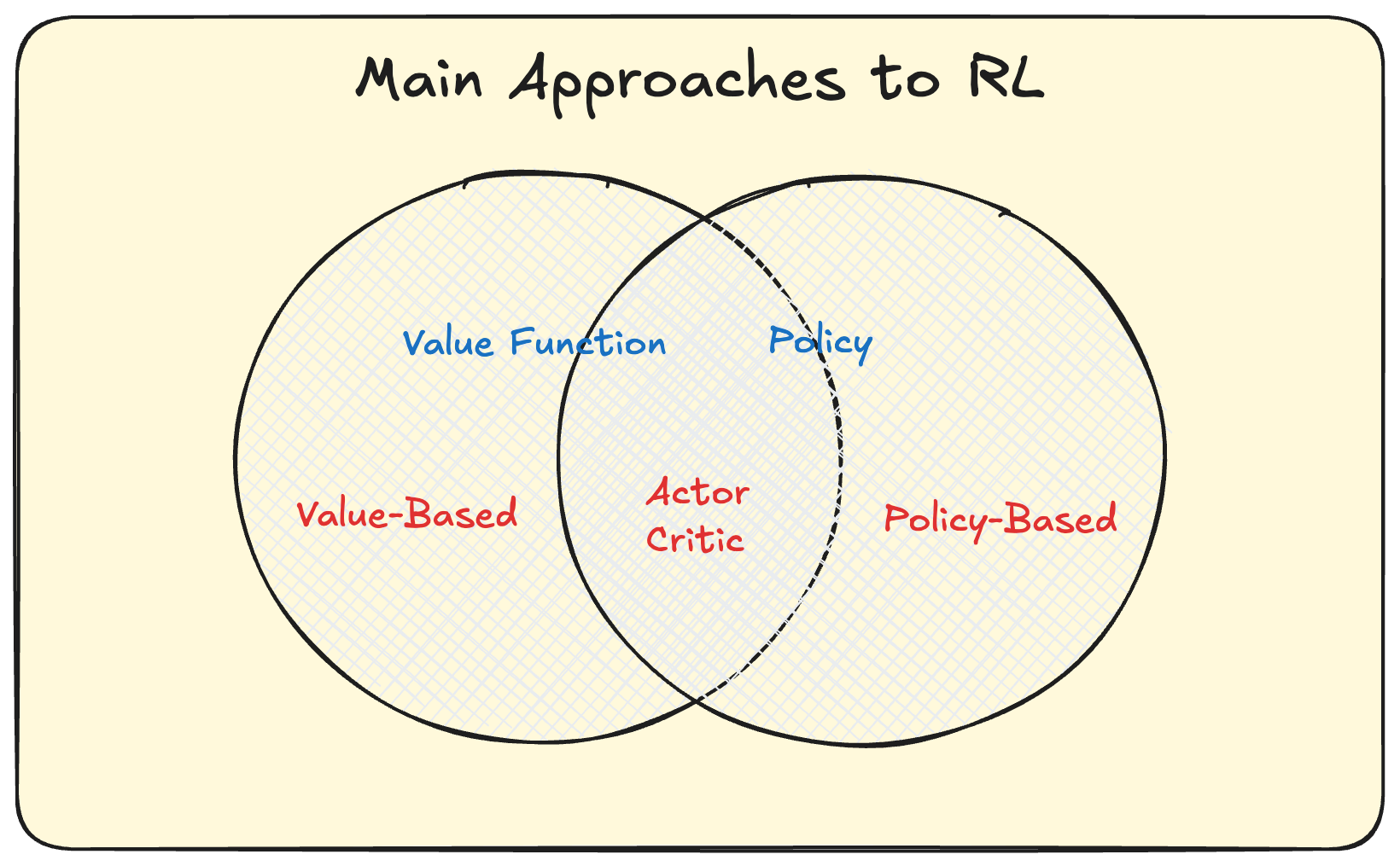
More concretely there are three main approaches to reinforcement learning: value-based, policy-based, and actor-critic methods. In value-based learning, we learn a value function \(Q_\theta(s, a)\) and infer a policy through maximization: \(\pi(s) = \arg\max_a Q(s, a)\). This approach uses an implicit policy. Policy-based learning takes a different route by explicitly learning the policy \(\pi_\theta(a \vert s)\) that maximizes reward across all possible policies, without maintaining a value function. Actor-critic methods combine both approaches by simultaneously learning both a value function and a policy, leveraging the benefits of each.
Role of the Actor
- Parameterizes the policy \(\pi_\theta(a \vert s)\), typically as a neural network that outputs a probability distribution over actions.
- Takes actions in the environment and is the only part that actually decides behaviour.
- Updates its parameters in the direction the critic’s feedback suggests.
Role of the Critic
- Learns a value function, usually the state value \(V_w(s)\), i.e. the expected return from a state under the current policy.
- Evaluates each action the actor took by comparing what happened against what it expected to happen.
- Provides that comparison as a low-variance feedback signal to the actor.
Why Bother? The Variance Problem
Combining policy and value-based approaches allows Actor-Critic methods to address some limitations of each individual approach, providing a more robust learning framework.
The motivation for using Actor-Critic methods stems from the challenges inherent in both value-based and policy-based RL. As Vapnik famously stated, “When solving a problem of interest, do not solve a more general problem as an intermediate step.” In the context of value-based RL, this suggests that learning a full value function can be unnecessarily complex when a simpler policy would suffice. On the other hand, pure policy gradient methods, such as REINFORCE, often suffer from high variance.
This variance issue arises because policy gradients estimate the expected reward by playing a game under the current policy and recording the states, actions, and rewards encountered. While this Monte-Carlo sampling approach provides an unbiased estimate, it can lead to high variance, meaning the policy updates might move in suboptimal directions. This in turn can make things even harder to recover from, since you then repeat the process with the updated policy which is now even further from the truth.
To illustrate, imagine playing \(N = 1000\) games, where the game is formalised as an RL problem, and plotting a histogram of the observed rewards; this typically results in a wide spread, which indicates high variance. If you were to then select a small sample of rewards, e.g. \(N = 5\), you’d likely notice a high degree of variability between them.
Actor-Critic methods aim to alleviate this variance by incorporating a critic to provide more stable and efficient feedback to the actor. In terms of the game analogy above, this would be like observing a distribution of estimated reward which has a slight bias yet is more peaked, and thus has lower variance.
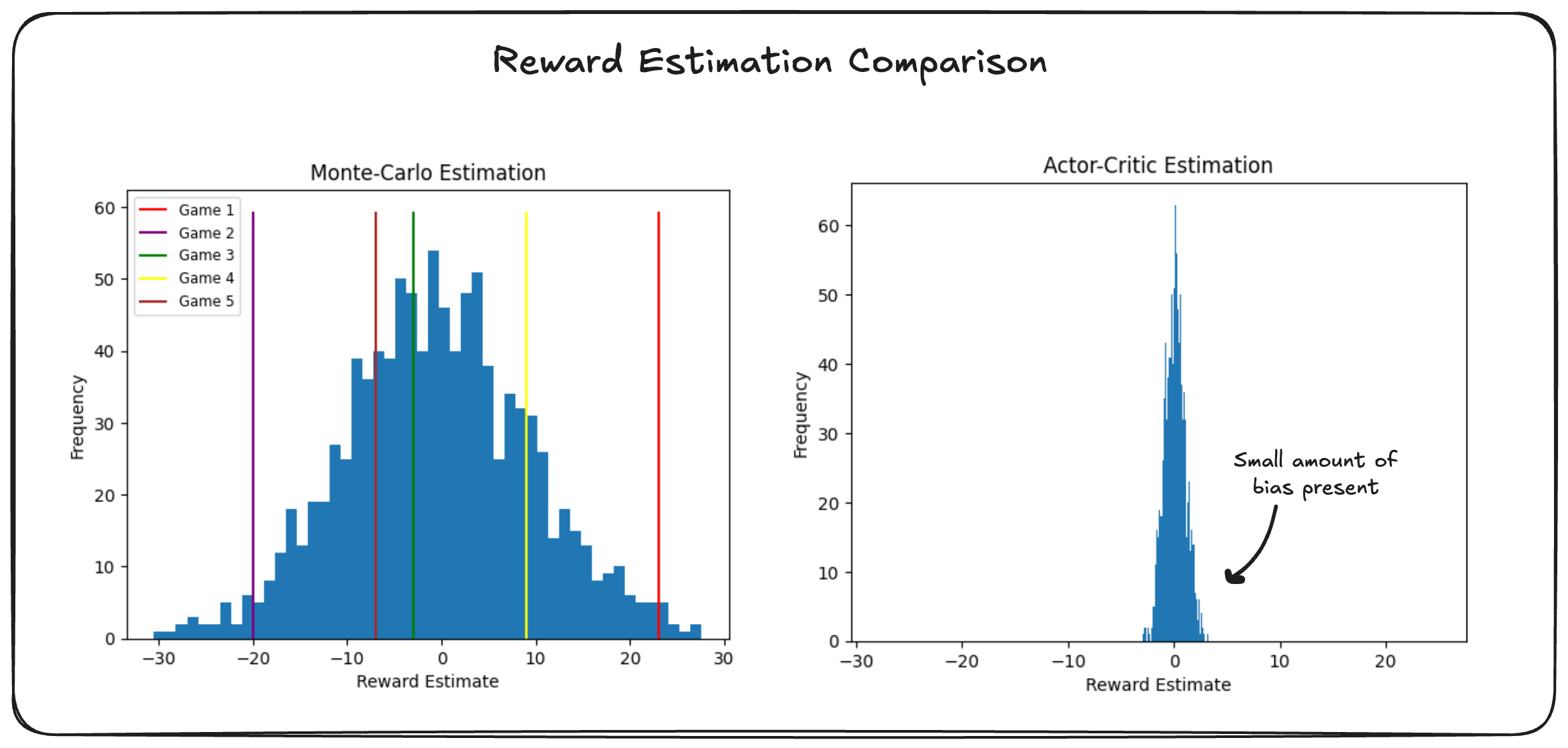
Don’t get too hung up on the exact choices of the plots themselves, they’re just shown to illustrate things.
Note: You can think of this stemming from the fact that the sample mean, used to estimate the expected reward, has its own expectation \(\mathbb{E}[\bar{X}]\) and variance \(\text{Var}(\bar{X})\). While increasing the number of games \(N\) can reduce the variance, it also increases the computational cost. Actor-Critic methods offer a way to reduce variance without such a steep increase in computation.
From REINFORCE to Actor-Critic in Four Steps
The critic can feel like it appears out of nowhere, so let’s build it up one small step at a time. In the policy gradients post we derived the REINFORCE estimator:
\[\nabla_\theta J(\theta) = \mathbb{E}_{\tau \sim \pi_\theta}\left[ \sum_{t=0}^{T} \nabla_\theta \log \pi_\theta(a_t \vert s_t) \, R(\tau) \right]\]Read it as: make the actions you took more likely, in proportion to the total reward you got. The problem is that \(R(\tau)\) is the return of one sampled trajectory, and a single noisy number multiplying every gradient term makes the whole estimate noisy.
Step 1: Subtracting a Baseline Changes Nothing (in Expectation)
Pick any baseline \(b(s)\) that does not depend on the action taken, and subtract it from the reward inside the estimator. The expected gradient is untouched, because for any fixed state \(s\):
\[\begin{aligned} \mathbb{E}_{a \sim \pi_\theta}\left[ \nabla_\theta \log \pi_\theta(a \vert s) \, b(s) \right] &= b(s) \sum_a \pi_\theta(a \vert s) \, \frac{\nabla_\theta \pi_\theta(a \vert s)}{\pi_\theta(a \vert s)} && \color{gray}\small\text{since } \nabla \log \pi = \tfrac{\nabla \pi}{\pi} \\ &= b(s) \sum_a \nabla_\theta \pi_\theta(a \vert s) && \color{gray}\small\text{the } \pi\text{'s cancel} \\ &= b(s) \, \nabla_\theta \sum_a \pi_\theta(a \vert s) && \color{gray}\small\text{swap sum and gradient} \\ &= b(s) \, \nabla_\theta 1 = 0 && \color{gray}\small\text{probabilities sum to 1} \end{aligned}\]The probabilities of all actions always sum to 1, and the gradient of a constant is zero. So replacing \(R(\tau)\) with \(R(\tau) - b(s)\) leaves the mean of our gradient estimate alone and only changes its variance. That is a free lunch: we get to choose \(b\) purely to make the estimate less noisy.
Step 2: The Best Baseline Is Roughly the Expected Reward
How much can a good baseline actually buy? Here is a toy problem small enough to compute exactly: a two-armed bandit with a 50/50 policy, where arm 1 pays out \(\mathcal{N}(3, 1)\) and arm 2 pays out \(\mathcal{N}(1, 1)\), so the expected reward is \(\mathbb{E}[R] = 2\). The single-sample gradient estimate is \(g = \nabla_\theta \log \pi_\theta(a) \,(r - b)\), and because the problem is tiny we can write its mean and variance in closed form for any baseline \(b\) (the figure below does exactly that, with seeded Monte-Carlo draws overlaid as a cross-check).
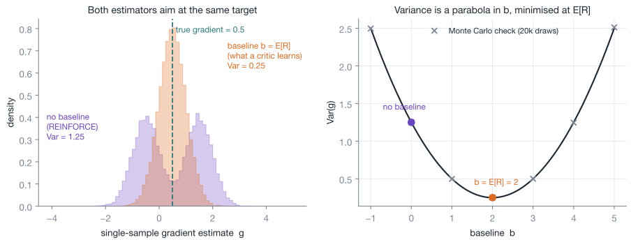
With no baseline the variance of \(g\) is 1.25; subtracting \(b = \mathbb{E}[R] = 2\) drops it to 0.25, an exactly 5x reduction, without moving the mean at all. And the right panel shows the variance is a parabola in \(b\) whose minimum sits at the expected reward, so “predict the reward you expect to get, then subtract it” is not just intuition, it is the (near) optimal choice. (Strictly, the exact minimiser weights each action’s reward by \(\pi(a)\,s(a)^2\), where \(s(a)\) is the score \(\nabla_\theta \log \pi_\theta(a)\); it coincides with \(\mathbb{E}[R]\) here because our 50/50 policy makes those weights equal, and in general it just sits close to it.)
Step 3: Let the Baseline Depend on the State. That’s the Critic
In a real RL problem the reward you should expect depends on where you are: being three moves from checkmate is not the same as the opening position. So the natural baseline is the state-value function \(V^\pi(s)\), the expected return from state \(s\) under the current policy. We don’t know it, so we learn it with a second network \(V_w(s)\). That network is the critic. Its entire job is to be a good baseline.
Once we subtract it, the quantity multiplying the gradient becomes the advantage:
\[A^\pi(s, a) = Q^\pi(s, a) - V^\pi(s)\]which asks: how much better was taking action \(a\) than what this policy usually achieves from state \(s\)? The policy update then becomes
\[\nabla_\theta J(\theta) = \mathbb{E}\left[ \nabla_\theta \log \pi_\theta(a \vert s) \, A^\pi(s, a) \right]\]and it has a satisfying reading: increase the probability of actions that did better than expected, decrease it for actions that did worse than expected, and leave alone actions that merely met expectations. Contrast that with REINFORCE, which happily reinforces a mediocre action just because the whole trajectory happened to score well.
Step 4: Estimate the Advantage with the TD Error
We can’t compute \(A^\pi(s,a)\) directly either, since it contains \(Q^\pi\). The standard trick is the one-step temporal-difference (TD) error:
\[\delta_t = r_{t+1} + \gamma V_w(s_{t+1}) - V_w(s_t)\]which compares what actually happened over one step (the reward plus the discounted value of where you landed) against what the critic predicted before the step. If \(V_w\) were the true value function, the TD error would be an unbiased estimate of the advantage:
\[\begin{aligned} \mathbb{E}\left[ \delta_t \mid s_t, a_t \right] &= \mathbb{E}\left[ r_{t+1} + \gamma V^\pi(s_{t+1}) \mid s_t, a_t \right] - V^\pi(s_t) && \color{gray}\small\text{plug in } \delta_t \\ &= Q^\pi(s_t, a_t) - V^\pi(s_t) && \color{gray}\small\text{Bellman equation} \\ &= A^\pi(s_t, a_t) && \color{gray}\small\text{definition of advantage} \end{aligned}\]That single scalar \(\delta_t\) now drives both updates, each with its own learning rate:
\[\begin{aligned} \text{critic:} \quad & w \leftarrow w + \alpha_w \, \delta_t \, \nabla_w V_w(s_t) \\ \text{actor:} \quad & \theta \leftarrow \theta + \alpha_\theta \, \delta_t \, \nabla_\theta \log \pi_\theta(a_t \vert s_t) \end{aligned}\]The critic moves its prediction toward what it just observed, and the actor shifts probability toward (or away from) the action, in proportion to how much of a positive (or negative) surprise it produced.
Note: This is where the bias sneaks in. During training \(V_w\) is not the true value function, so bootstrapping off its estimate of the next state injects some bias in exchange for the big variance reduction, which is exactly the peaked-but-slightly-shifted distribution we sketched earlier. Methods like Generalized Advantage Estimation (GAE) expose this as a dial, blending one-step TD errors (low variance, more bias) with full Monte-Carlo returns (no bias, high variance).
Key Components
Actor Network
- Architecture: typically a neural network.
- Function: parameterizes the policy, outputting action probabilities (or a deterministic action in continuous-control variants).
Critic Network
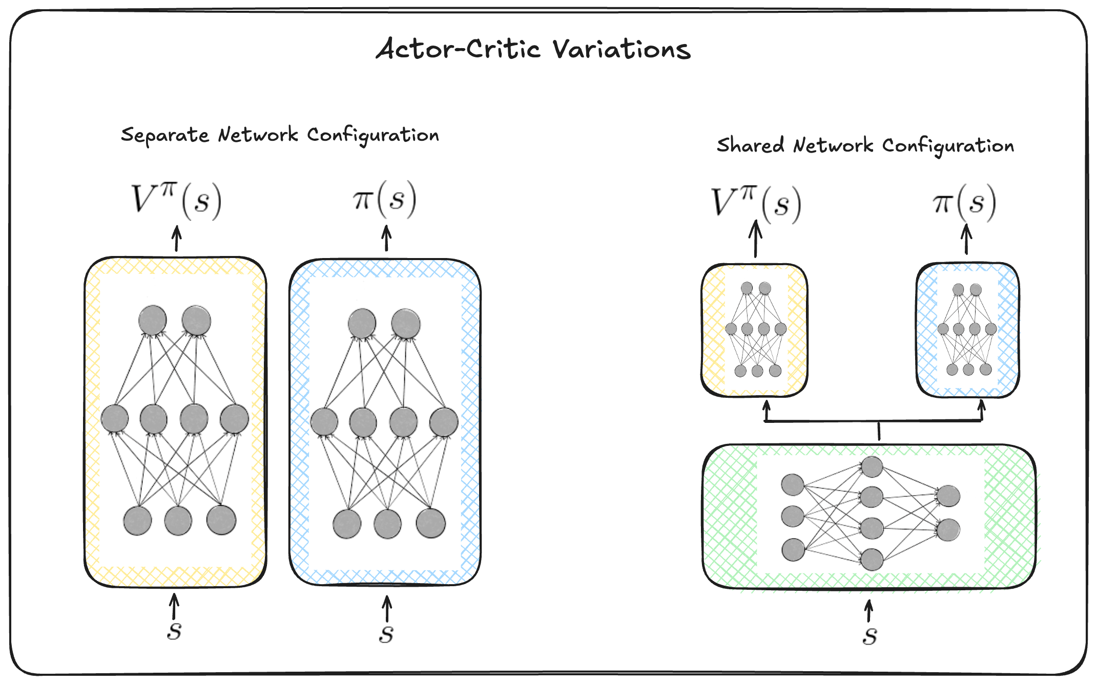
- Architecture: typically a neural network, often sharing early layers with the actor since both need to understand the state.
- Function: estimates the value function (e.g. Q-value or state-value).
Sample implementation for the CartPole environment, adapted from the PyTorch examples repo. The two heads share a body: 4 state inputs (cart position/velocity, pole angle/velocity), 2 action outputs (push left or right), and 1 value output:
import torch.nn as nn
import torch.nn.functional as F

class Policy(nn.Module):
    """
    implements both actor and critic in one model
    """
    def __init__(self):
        super(Policy, self).__init__()
        self.affine1 = nn.Linear(4, 128)

        # actor's layer
        self.action_head = nn.Linear(128, 2)

        # critic's layer
        self.value_head = nn.Linear(128, 1)

        # action & reward buffer
        self.saved_actions = []
        self.rewards = []

    def forward(self, x):
        """
        forward of both actor and critic
        """
        x = F.relu(self.affine1(x))

        # actor: choses action to take from state s_t
        # by returning probability of each action
        action_prob = F.softmax(self.action_head(x), dim=-1)

        # critic: evaluates being in the state s_t
        state_values = self.value_head(x)

        # return values for both actor and critic as a tuple of 2 values:
        # 1. a list with the probability of each action over the action space
        # 2. the value from state s_t
        return action_prob, state_values
The update step is where the math from the previous section becomes code. Acting means sampling from the actor’s distribution and remembering both the log-probability (for the actor update) and the critic’s value estimate (for the baseline):
from collections import namedtuple
import torch
from torch.distributions import Categorical

SavedAction = namedtuple('SavedAction', ['log_prob', 'value'])

def select_action(state):
    state = torch.from_numpy(state).float()
    probs, state_value = model(state)

    # sample an action from the actor's distribution pi(a|s)
    m = Categorical(probs)
    action = m.sample()

    # stash log pi(a|s) and the critic's V(s) for the update step
    model.saved_actions.append(SavedAction(m.log_prob(action), state_value))
    return action.item()
And at the end of each episode both losses are computed from the same stored quantities:
def finish_episode():
    R = 0
    saved_actions = model.saved_actions
    policy_losses = []  # actor:  -log pi(a|s) * advantage
    value_losses = []   # critic: regression of V(s) onto the observed return
    returns = []

    # walk backwards to compute the discounted return G_t at every step
    for r in model.rewards[::-1]:
        R = r + gamma * R
        returns.insert(0, R)
    returns = torch.tensor(returns)
    returns = (returns - returns.mean()) / (returns.std() + eps)

    for (log_prob, value), R in zip(saved_actions, returns):
        advantage = R - value.item()          # A_t = G_t - V(s_t)

        policy_losses.append(-log_prob * advantage)
        value_losses.append(F.smooth_l1_loss(value, torch.tensor([R])))

    optimizer.zero_grad()
    loss = torch.stack(policy_losses).sum() + torch.stack(value_losses).sum()
    loss.backward()
    optimizer.step()

    del model.rewards[:]
    del model.saved_actions[:]
Two details worth noticing. First, the advantage line uses value.item(), which detaches the critic from the actor’s loss: the actor treats the baseline as a constant, exactly as the math assumed, and the critic is trained only by its own regression loss. Second, this particular implementation uses the full Monte-Carlo return \(G_t\) as the critic’s target and \(G_t - V_w(s_t)\) as the advantage, which is the simplest batch flavour; swapping in the TD error from step 4 gives the fully online version that updates at every step.
The Algorithm Loop
- The actor takes an action based on the current policy.
- The critic evaluates the outcome and computes the TD error.
- The actor updates its policy in the direction the TD error suggests.
- The critic updates its value function to better predict future rewards.
Variants of Actor-Critic Methods
The actor-critic skeleton shows up, with different dressing, in most of the well-known deep RL algorithms:
- A2C (Advantage Actor-Critic): essentially the recipe derived above, run synchronously over a batch of parallel environments so gradient updates average over many streams of experience.
- A3C (Asynchronous Advantage Actor-Critic): many worker copies of the agent explore their own environments and update a shared set of parameters asynchronously, which both speeds up and decorrelates learning.
- DDPG (Deep Deterministic Policy Gradient): extends the idea to continuous action spaces with a deterministic actor and a Q-function critic, borrowing experience replay and target networks from DQN.
- TD3 (Twin Delayed DDPG): patches DDPG’s tendency to overestimate values by training two critics (taking the more pessimistic one) and updating the actor less frequently than the critics.
- SAC (Soft Actor-Critic): adds an entropy bonus so the actor is rewarded for staying stochastic, improving exploration and robustness in continuous control.
- PPO (Proximal Policy Optimization): an advantage actor-critic with a clipped objective that stops any single update from moving the policy too far; its simplicity and reliability have made it the default choice in many settings, including aligning large language models with human feedback (RLHF).
The baseline idea itself is still evolving: GRPO, the method behind DeepSeek’s math-reasoning models, drops the learned critic entirely and instead uses the average reward of a group of sampled answers to the same prompt as the baseline, a reminder that the critic was only ever there to estimate expected reward.
Applications
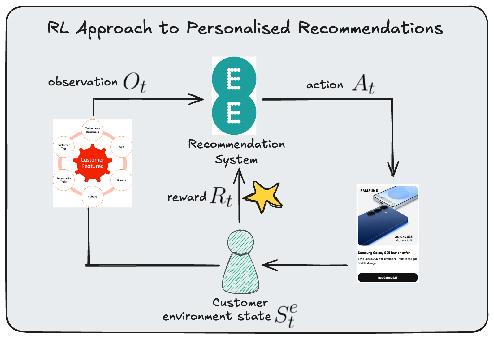
Actor-Critic methods are used in various real-world applications, including robotics, game playing, and autonomous driving, and most notably for providing personalised recommendations to customers.
Conclusion
Actor-Critic methods combine the strengths of value-based and policy-based approaches: the actor keeps the directness of policy gradients, and the critic supplies a learned baseline that tames their variance at the cost of a little bias. That bias-variance dial, from full Monte-Carlo returns down to one-step TD errors, is the single most useful mental model for navigating the whole family, and once you see it, algorithms like A2C, DDPG, SAC and PPO stop looking like separate inventions and start looking like different settings of the same few knobs.
Further Resources
- Research Papers
- Foundational Papers
- Barto, Sutton & Anderson (1983): Actor-Critic Architecture
- Sutton et al. (2000): Policy Gradient Methods
- Deep RL Advances
- Mnih et al. (2016): A3C
- A breakthrough in deep RL. A3C trained multiple actor-critic agents in parallel threads, achieving state-of-the-art results on Atari games and continuous control tasks. This paper demonstrated the stability and efficiency gains from using an actor-critic with multi-threaded training.
- Lillicrap et al. (2015): DDPG
- An actor-critic algorithm for continuous action spaces. DDPG uses a parametric actor (policy network) and a critic (Q-value network), along with experience replay and target networks (inspired by DQN), to learn continuous control policies (e.g. for robotic locomotion). It became a foundation for many continuous RL methods.
- Schulman et al. (2015): GAE
- Generalized Advantage Estimation, the paper behind the bias-variance dial mentioned above: it interpolates between one-step TD errors and full Monte-Carlo returns with two parameters.
- Schulman et al. (2017): PPO
- PPO is a widely used policy optimization method that can be seen as an actor-critic approach (with a clipped surrogate objective) for stability. It simplifies earlier trust-region methods while achieving robust performance. PPO’s popularity in the RL community is due to its ease of use and reliability on a variety of benchmarks.
- Haarnoja et al. (2018): SAC
- Introduced Soft Actor-Critic, an off-policy actor-critic algorithm that maximizes a trade-off between expected reward and entropy. SAC’s stochastic actor aims for both high reward and high randomness (exploration), leading to state-of-the-art results in continuous control. This represents a recent advancement in actor-critic methods, improving stability and sample efficiency.
- Mnih et al. (2016): A3C
- Application in Recommendation Systems
- Survey (Lin et al., 2021): Reinforcement Learning for Recommender Systems
- Zhao et al. (2019): Deep RL for List-wise Recommendations
- Chen et al. (2019, YouTube/Google): Top-K Off-Policy Correction
- Xin et al. (2022): Supervised Advantage Actor-Critic
- Hierarchical Actor-Critic for Recommendations: Recent Research
- Foundational Papers
- Articles, Tutorials, and Blogs
- Lilian Weng’s Blog: Policy Gradient Algorithms (Actor Critic)
- Hugging Face’s Deep RL Course: Actor-Critic Unit
- Chris Yoon’s Tutorial: Understanding A2C
- OpenAI Spinning Up: RL Documentation
- Great for learners trying to upskill more broadly in the field of deep rl. Includes readable introductions to policy gradient and actor-critic approaches. For example, it features sections on Vanilla Policy Gradient (REINFORCE), A2C/A3C, DDPG, PPO, and SAC, along with code snippets.
- Implementations and Code Examples