Table of Contents
- Representing Products with Features
- Visualizing Product Similarity with UMAP
- Performance Testing and Experimental Approach
- Potential Future Developments
- Conclusion
- Resources
When an online shopper views a product, it’s essential to show them other items that are similar – often labeled “More Like This” or “Similar Products.” These recommendations help users discover related products and keep them engaged. One effective way to build such a recommender is by using a content-based approach, which relies on product attributes (content) rather than user behavior. A content-based model finds look-alike items based on features like category, brand, or description, making it a great starting point for recommendation systems, especially if historical interaction data is limited.
Why start with a content-based model? In scenarios where user interaction data is sparse or new products lack engagement history, content-based recommendations can still provide relevant suggestions. They leverage information about the items themselves. This means even a brand-new item with no sales or ratings can be recommended to users if it shares characteristics with other items. Content-based methods thus help address the “cold-start” problem – new users or items with limited interaction history can still receive meaningful recommendations (Introduction to recommender systems). As one expert observed, “the only time to rely on content-based recommendations is when your catalog is of one-off items, which never get enough [collaborative filtering] interactions or you have rich content.” (machine learning - Recommender System: Is it content-based filtering? - Stack Overflow). This highlights that content-based techniques are crucial when behavioral data is insufficient yet you still have rich product information. In contrast to collaborative filtering (which needs plenty of user behavior data to find patterns), a content-driven approach can start delivering value from day one by using product data that’s already available.
In the rest of this post, the following sections outline a general approach to building a ‘Similar Products’ recommender using content-based techniques. We will cover how to represent products with features, how to measure similarity with customizable weighting, how to retrieve and rank similar items, and how to incorporate business rules into the recommendation process. We’ll also discuss visualizing the product space using a dimensionality reduction technique (UMAP) to ensure the model is capturing intuitive similarities along with an approach for testing the system once developed. The goal is to present the approach in a general way, so it can be adapted to various contexts and datasets.
Representing Products with Features
The first step in a content-based recommender is to represent each product as a set of features. Each product is characterized by its attributes, which serve as the building blocks for measuring similarity. Common features used can include:
- Category and sub-category – e.g., a product’s taxonomy or type (a running shoe vs. a dress).
- Brand – products from the same brand might be considered more similar in certain business contexts.
- Specifications - detailed list of specs for product provided by manufacturers (e.g computer chip models, fabric used in clothes etc).
- Text descriptions – detailed handwritten description provided by product marketing/proposition teams.
- Other attributes – such as colour, price and other metadata about the product.
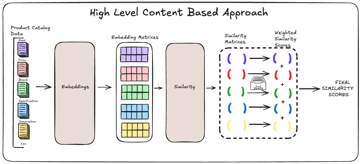
These features can be encoded in vector form for each item. For example, categories and brands might be one-hot encoded (or represented in an embedding space), textual data might be transformed into a numeric vector using NLP techniques, and numeric features like price can be normalized. The end result is that each product lives in a feature space where similarity can be quantified: the more overlapping or closer the features, the more similar two products are in this space.
Weighted Similarity Scoring
Not all features are equally important. In this approach, each feature (or group of features) is given a weight reflecting its importance in defining “similarity.” The model computes a similarity score for each feature separately, then combines them in a weighted manner. Here’s how it works:
- Feature-level similarity: For each feature, define a way to measure how similar two products are on that attribute. For example, for brand, the similarity could be 1 if the brands match (and 0 otherwise). For a numeric attribute like price, the similarity could be a function that decreases as the price difference increases. For text features, cosine similarity between text embedding vectors can quantify how alike two descriptions are.
- Normalized weights: Assign a weight to each feature (or feature type) based on its importance. These weights are normalized (for instance, summing up to 1.0) so that each feature’s contribution is proportional. For example, brand might have weight 0.3, category 0.4, description text 0.2, and price 0.1 – indicating category is deemed most important, followed by brand, etc. (These numbers can be tuned.)
- Combined score: The model calculates an overall similarity between a query product and a candidate product by summing up the feature-level similarities multiplied by their respective weights. In formula form, if the features are $f_1, f_2, …, f_n$ with weights $w_1,…,w_n$, and $\text{sim}_i(A,B)$ is the similarity of products A and B on feature $i$, then:
\(\text{Similarity}(A,B) = \sum_{i=1}^{n} w_i \times \text{sim}_i(A,B).\)
This yields a weighted similarity score that accounts for each aspect of the product.
By adjusting the weights, the recommendation engine can be tuned to align with business intuition. If brand consistency is very important (say customers looking at Nike shoes should see mainly Nike recommendations), the weight for the brand feature can be increased. If more diversity is desired, weights can be balanced to not overemphasize any single attribute. This flexibility in weighting is one of the strengths of a content-based approach in a business setting, as it allows quick iteration and alignment with domain expertise without retraining a complex model.
Retrieving Similar Products with Nearest Neighbors
Once products are encoded and we can compute similarity scores, the next step is to efficiently find the most similar items for any given product. The straightforward way is to compare the query product to every other product, compute all the similarity scores, and then pick the top results. However, doing a brute-force comparison for each query can become slow if the catalog is large. Instead, we can use a nearest neighbors search to speed this up.
A potential “out of the box” approach employs scikit-learn’s NearestNeighbors algorithm to handle the similarity search. This tool allows precomputing data structures for the item feature vectors and then quickly querying for the nearest neighbors (the items with highest similarity) of a given product (K-NN vs Approximate Nearest Neighbors - Sefik Ilkin Serengil). In essence, the algorithm “remembers” all product vectors; given a query product, it efficiently finds which items are closest in the feature space. Because the feature weights are incorporated into the similarity calculation (either by scaling the features in the vectors or via a custom distance metric), the NearestNeighbors results reflect the intended weighted similarity measure.
Notably, this approach uses an exact K-Nearest Neighbors search rather than an approximate one. Approximate Nearest Neighbor (ANN) methods (like those in libraries such as Faiss or Annoy) can dramatically speed up searches in very large datasets by allowing a slight trade-off in accuracy. In this scenario, the product catalog and feature set were manageable enough that an exact search was preferable to ensure accuracy. As a rule of thumb, exact k-NN is suitable for small to moderate-sized datasets when precise similarity rankings are required and the search time is acceptable. In other words, k-NN provides exact results, but can be computationally expensive as the dataset grows; if the catalog had been in the millions of items, an ANN approach might be warranted, but that wasn’t necessary in this case.
Under the hood, scikit-learn’s NearestNeighbors can use algorithms like brute-force search or ball-tree/kd-tree structures to find neighbors efficiently. With our weighted similarity, one practical method is to precompute a composite feature vector for each item that accounts for the weights (for example, scaling each feature dimension by its weight). Then a standard distance metric (like euclidean or cosine distance) can be used by NearestNeighbors to fetch the top matches. Alternatively, the similarity scores could be computed feature-by-feature on the fly for a set of candidate neighbors if needed. Either way, the retrieval step produces a list of candidate products that are most similar to the query item by content features.
Business Rules and Ranking with Metadata
Finding similar items by attributes is a great start, but in a production environment, not every “similar” item can be shown as a recommendation. There are often business rules and constraints that determine the pool of eligible recommendations for a given product page or context. This is where a final filtering and ranking step comes in.
In practice, an internal platform or business logic layer might pre-filter which products are allowed to appear as “similar items” for a given target product. For example, the business may require that out-of-stock items are excluded, or that certain categories (like clearance products) only recommend other clearance products. There could also be rules such as only show similar items from the same organisation, to keep recommendations contextually relevant. Because of these constraints, the recommender system doesn’t simply take the top N nearest neighbors from the entire catalog; instead, it narrows the candidates to those that pass the business criteria first.
This step is responsible for taking the similarity-ranked candidates and applying these business-driven filters and ordering. Essentially, it intersects the set of top similar items with the set of allowed/eligible items for that context, and then ranks that final list (often by the similarity score) which can be thought of as a form of “masking recommendations”. This two-step approach – first generate candidates by similarity, then filter and sort them by business rules – ensures the recommendations not only make algorithmic sense but also meet practical business requirements. It’s common in industry to apply such business rules either before or after the recommendation algorithm does its work (named entity recognition - How to filter Items in Recommender Systems? - Data Science Stack Exchange).
An added benefit of the weighted-feature approach described earlier is how easily the ranking can be tweaked to satisfy business goals. Because each feature’s influence is explicit and adjustable, product teams can calibrate the recommendations by tuning weights rather than retraining models. For instance, if the team decides that brand should have even more influence on the final shown products (perhaps to promote brand loyalty or a consistent style), they can increase the brand weight in the similarity calculation. The next time recommendations are generated, items sharing the same brand will score higher and thus rank higher among the eligible results. This business-driven ranking approach, powered by flexible feature weightings, means the system can respond quickly to strategy changes. Ultimately, the final set of recommendations for a product page is determined by this ranking step – ensuring every item shown is both content-similar and compliant with the business’s display criteria.
Visualizing Product Similarity with UMAP
To interpret the results and verify that the model is capturing intuitive similarities, a dimensionality reduction technique called UMAP (Uniform Manifold Approximation and Projection) can be employed to project the high-dimensional item vectors down to two dimensions for visual analysis. UMAP is well-suited for this task because it is designed to preserve local structure (i.e. items that are close in the original feature space stay close in the low-dimensional projection), and it tends to handle larger datasets more efficiently than the older t-SNE method (T-sne and umap projections in Python). In fact, UMAP is “a dimensionality reduction [technique] specifically designed for visualizing complex data in low dimensions (2D or 3D)” much like t-SNE, but with better runtime scalability as data grows (T-sne and umap projections in Python).
In the 3D UMAP visualization of the products, each point represents a product, plotted such that distances between points reflect their content-based similarity. The outcome was insightful: the plot revealed clear clusters of similar items. For example, products in the same category often formed tight groups in the 3D space — all the running shoes clustered in one area while formal leather shoes clustered in another, reflecting that the content features (like category and text descriptors) indeed group those items together. Similarly, items from the same brand bunched together when brand was a significant factor in the similarity score. This visual confirmation indicates that the model isn’t producing arbitrary results; rather, it’s grouping products in a way that aligns with human intuition about product similarity.
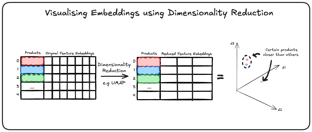
Such visualizations can also communicate to non-technical stakeholders how the recommendation system “sees” the product catalog. It turns abstract vector math into a tangible map. Stakeholders can observe, for instance, that winter coats are all located near each other (and not mixed with summer T-shirts), which builds confidence that the model is capturing the right notions of similarity according to domain knowledge.
Performance Testing and Experimental Approach
Performance testing should be tailored to the specific problem and context. When deploying a new system, it’s crucial to assess the overall value contribution, not just the model’s performance in isolation.
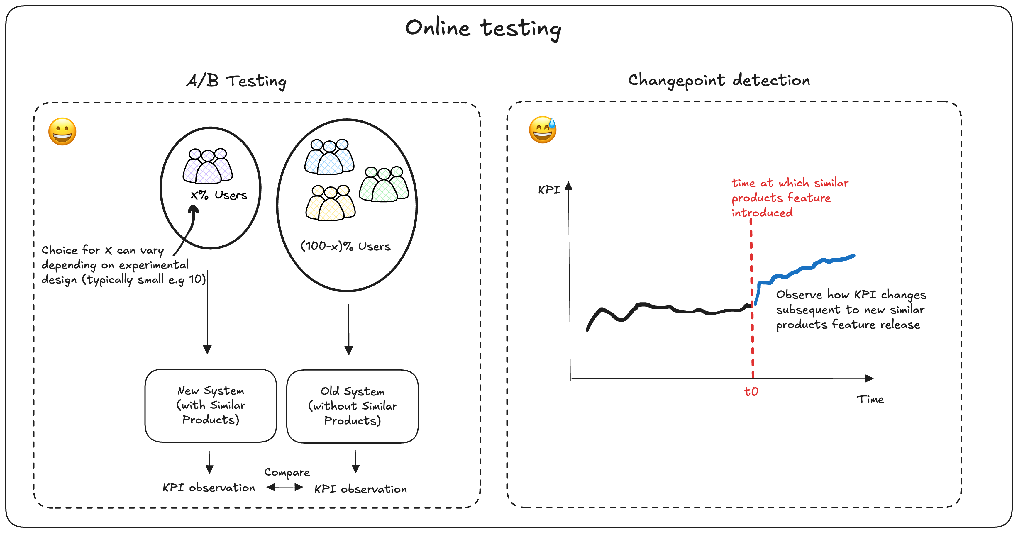
Given the business problem discussed so far, we plan to use the following experimental methods:
- Step 1: Determine if we can set up an A/B test to compare the existing experience with the new, model-augmented experience.
- A/B tests should be designed to answer a specific question, such as “What is the value of deploying a similar products model?”. Therefore, we would test “having a carousel vs. not having a carousel.”
- Given our intuition that this model will be beneficial, a 90/10 split may be appropriate, allowing the majority of users to benefit from the new experience. A 50/50 split is not necessary.
- Step 2: If an A/B test isn’t feasible, we could instead perform a quasi-experiment. This involves deploying the model and tracking relevant metrics (e.g., add to basket, purchases, and clicks). Change point detection can then be used to assess the value added.
- There is a risk that other unknown factors or events could influence these metrics (e.g., seasonal impact, other marketing campaigns, or external news events).
- Step 3: Step 2 should provide sufficient short-term performance data. Over time, as the system/model is iterated upon, a challenger baseline approach can be used to further measure performance. For example, how does new model X (using business rules, ML, etc.) compare to our currently implemented model? What is the incremental value?
Potential Future Developments
Several avenues exist for future work to enhance the system:
- Feature Engineering & Model Enhancements: As more data becomes available, consider incorporating additional modalities such as images or user behavioral data. For instance, visual features could be extracted from product images using a CNN. Currently, feature weights (categorical, numerical, textual) are fixed. A potential improvement is to learn these weights from data (e.g., via meta-learning or a small neural network) so that the system can better adapt to feature importance over time.
- Improved Textual Representations: Experiment with different sentence transformer models (or even domain-specific fine-tuning) to improve the quality of textual embeddings. As data grows, consider models that capture context better (e.g., using models like BERT variants fine-tuned on product descriptions or other SOTA transformer based encoder models).
- Similarity Computation: For larger catalogs, consider using libraries like FAISS, Annoy, or HNSWlib which provide faster approximate nearest neighbor searches. Experiment with hybrid similarity metrics that combine multiple distances or even use metric learning to tailor the distance measure based on historical recommendation success.
- Model Training: Currently, when a new variant is added, the nearest neighbor models are refit entirely. In a production scenario with a large or streaming dataset, consider incremental updating methods or using libraries that support online learning. As user interactions with the recommendations are recorded, integrate this feedback to adjust models or feature weights dynamically.
Conclusion
Building a ‘Similar Products’ recommender with a content-based approach provides a strong baseline for product recommendations, especially in data-sparse environments. By leveraging product attributes and a weighted similarity scheme, the system can generate relevant recommendations even for new or niche items. This method is transparent (recommendations can be explained by pointing to product features) and adaptable – one can reweight features or incorporate new attribute data as business needs evolve.
Moreover, layering business rules in the recommendation pipeline ensures the results make sense not just algorithmically but also in terms of real-world business constraints (showing only appropriate and available products to customers). The UMAP visualization confirmed that the model’s notion of “similarity” largely aligns with human intuition, which is crucial for gaining stakeholder buy-in and trust.
As a next step, once more user interaction data becomes available, one could enhance this content-based foundation with collaborative filtering or hybrid approaches to further improve the recommendations. Nonetheless, a content-based strategy is an excellent starting point and a reliable component in situations where user-behavior data is sparse. By following the approach outlined above, teams can deliver an engaging “similar products” feature that improves user experience and drives product discovery, all while maintaining the flexibility to adjust to business priorities.
Resources
For those interested in learning more about the concepts behind this system, here are some useful articles and blog posts on recommendation systems, embeddings, and nearest-neighbor search:
- What are Vectors?
- Simple mathematical description of vectors, useful in helping contextualise things discussed in this post. The following video also provides and excellent overview, see here.
- What are Embeddings? – An accessible explanation of embeddings, how they are created, and why they’re useful in machine learning, with examples across text, images, and more.
- Understanding UMAP
- Neat blog post which provides useful visuals to help explain the inner workings of UMAP.
- What is Nearest Neighbor Search in Embeddings? – Introduction to how nearest neighbor search works with embeddings, covering brute-force vs. optimized methods and use cases in recommendations.
- Using Auto-Encoders to Find Similar Items – A case study of using an autoencoder-based approach for content-based recommendations, similar to our approach of learning item embeddings for similarity.
- Item2Vec: Neural Item Embeddings to Enhance Recommendations
- Explores the use of neural embeddings (inspired by word2vec) to capture product similarities. This article is valuable for learning how deep learning approaches can be applied to generate item representations for enhanced recommendation systems, making it a relevant read for product similarity topics.
- Item-Item Recommendation with Surprise
- Provides a practical walkthrough of building an item-item recommendation system using the Surprise library in Python. This resource is useful for understanding traditional collaborative filtering techniques and implementing product similarity measures in a hands-on manner.