Intro
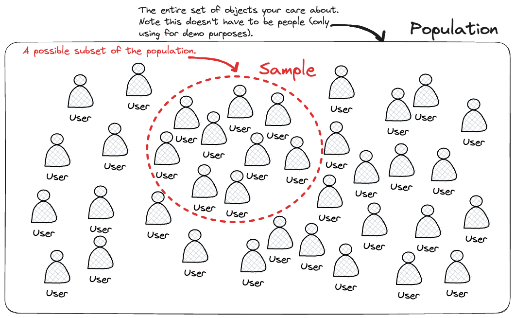
Say you have a population represented by your entire dataset and you want to understand things about it, often times you don’t have the time or resources to calulate things based on all of that data. In this scenario your hopes are that you can take a sample (ie a subset of your dataset) calculate somethings on it and then infer the behavoiur of your population based on this.
This is at the core of why you would want to perform sampling.
Jargon defintions
Statistics has many defintions in general so it’s important to understand what these are encase you encounter them when reading different literature.
- Bootstraping:
- Act of performing multiple resamples (sampling with replacements) of the same size as your intial data to generate a theortical distribution of the underlying populating. In some sense it is the opposite of traidtional sampling whereby you select a smaller subset of your starting data since instead you create a boostrap sample of the same size as your intial data.
- Code wise something like
df.sample(frac=1, replace=True)pandas docs for sample method contains more info.
- Sampling:
- Usually this refers to taking a subset of the data that you have to begin with. Most texts usually consider this as sampling without replacement but it’s important to check.
- Simple random sampling is an example of this.
- Code wise something like
df.sample(n=10, random_state=SEED)selects a sample of 10 entries from your data (assuming you have more than 10 records). Equally you could use thefracarguement to select a proportion, main noteworthy point is the.samplemethod by default setsreplace=Falsehence sampling without replacement.
- Probability Density Function:
- A function corresponding to the probability distribution associated with a continous random variable. This depends on the theoretical distribution used to model your random variable.
- Usually represented like $P(X = x)$ where $X$ is your random variable and $x$ represents a particular value of your variable.
- You can kind of think of it as the smoothed equivalent of a histogram where the area under the curve represents the probability with the following properties.
- $f(X) \ge 0$ (cannot have a negative probability)
- $P(a < X < b) = \int_{a}^{b} f(x) dx$ (probability between values is the area between them).
- $\int_{-\infty}^{+\infty} f(x) dx = 1$ (total probability equals one).
- Point estimate:
- Sometimes called an estimate too.
- Represents a value used to approximate a population parameter.
- Calculated from a particular sample (could be the average over a sampling distribution or bootstrapped distribution or just a single sample itself).
- Cumulative Density Function:
- Can get this from the p.d.f by summing all values less than or equal to a particular value.
- Like $F(x) = P(X \le x) = \int_{- \infty}^{x} f(t) dt$ where $f(t)=f(x)$ ie your p.d.f and we are using $t$ as a dummy variable.
- Can get this from the p.d.f by summing all values less than or equal to a particular value.
So, that being said what are the various types?
Many types of sampling exist but the most common ones have been added below.
- Simple Random Sampling
- Typically when you are randomly selecting members of your population sample without replacement.
- In pandas it can look something like
df.sample(n=N_SAMPLES, random_state=SEED)if you want to select a fixed number ordf.sample(frac=SAMPLE_FRACTION)if you want to select a particular fraction of observations
- Systematic Sampling
- Typically when you are sampling using a specfic rule with a fixed sample size in mind.
- In pandas something like
df.iloc[::interval, :]wheresample_steps=N_STEPS & pop_size=len(df)sointerval = pop_size // sample_steps.- This ensures that you are ensuring you get as many samples as possible.
- You should only use this methods if no patterns are present in your data.
- Otherwise this method will “remove” these inherent patterns crucial to understanding your data.
- Stratified Sampling
- Typically used when you want to ensure a particular data fields distribution is maintained in the resulting sample.
- Note otherwise typically there is a chance that your sample doesn’t contain any of a particular field (by chance). This isn’t always an issue but is if you want to study that particular field using your sample.
- Steps are to split the population into these subgroups and then simple random sample on every subgroup.
- In pandas python you can chain together both the
.groupbyand.samplemethod to get the desired result. Something likedf.groupby("grouping_field").sample(frac=SAMPLE_FRACTION, random_state=SEED). You could instead specify the number of samplesn=N_SAMPLESinstead of thefracarguement which would eliminate the chance of getting a different proportions across the groups (since otherwise you don’t know how many samples are in each group).- Under the hood the
.groupbycreates an intermediate object which has a lazy evaluation policy, meaning no computation is performed until the.samplemethod is called (more efficient) which then selects the desired proportion/samples from each of the unique group combinations.
- Under the hood the
- Typically used when you want to ensure a particular data fields distribution is maintained in the resulting sample.
- Weight Random Sampling
- Similar to simple random sampling except you specify weights which can adjust the relative probability of particular rows being sampled
- Intuitvely can think of it as scaling the probability of sampling by that weight factor.
- This can be extrememly useful if you’d like to increase the representation of a particular set of rows in your sample.
- You can customize the weight creation field how you want, this provides freedom in exactly how each column is scaled up.
- In pandas you can create say some numeric column say by a condition and then specifcy that column to the
weightargument of the.samplemethod. Something likedf.sample(frac=SAMPLE_FRACTION, weight="weight_column_name")
- Similar to simple random sampling except you specify weights which can adjust the relative probability of particular rows being sampled
- Cluster Sampling
- Similar to stratified sampling except you simple random sample to select your sub groups & then perform simple random sampling only on those subgroups.
- In theory you’d only want to perform this if computational costs or time taken are too high to perform standard stratified sampling.
- In pandas something like:
unique_sub_groups = list(df["grouping_field"].unique())to get the unique sub groups that you want to sample from.sample_sub_groups = random.sample(unique_sub_groups, k=N_SAMPLES)to sampleN_SAMPLESfrom the unique list of sub groups utilising the built inrandommodule.filtering_condition = df["grouping_field].isin(sample_sub_groups)followed bydf_cluster = df.loc[filtering_condition]to remove records not in our condition.df["grouping_field"] = df["grouping_field"].cat.remove_unused_categories()to remove any categories which aren’t in our condition to avoid errors when sampling.df.groupby("grouping_field").sample(n=N_SAMPLES, random_state=SEED)to now just performing grouping on this field and sample how many we want.
- Similar to stratified sampling except you simple random sample to select your sub groups & then perform simple random sampling only on those subgroups.
How can you create your own sampling distribution
The idea here is to perform your sampling technique on your data and subsequently calculate a statistic on that sampled data (summarising the data however you want) and then proceding to perform this multiple times. By doing these you’ll build up a set of values which you can then be plotted to showcase the distribution.
Naively something like this works:
import matplotlib as plt

N_SAMPLES = 100
SAMPLE_SIZE = 50
DESIRED_VARIABLE = "some variable"
N_BINS = 10
simple_random_sample_means = []

# Looping over to generate multiple samples
for i in range(N_SAMPLES):
    simple_random_sample_means.append(
        # Performing the sampling itself and calculating desired metric
        df.sample(n=SAMPLE_SIZE)[DESIRED_VARIABLE].mean()
    )

# Plotting distribution which takes array like inputs and the bins you'd want
plt.hist(sample_means, bins=N_BINS)
plt.show()
Where your desired statistic is a mean over the desired variable of choice in your dataset and your sampling technique is simple random sampling. This can then be plotted, assuming you’re dealing with a continous random variable a histogram is a good plot to showcase distributions.
If instead you wanted to perform boostrapped distribution you could perform nearly identical steps as shown below
import matplotlib as plt

N_SAMPLES = len(df)
SAMPLE_SIZE = 50
DESIRED_VARIABLE = "some variable"
N_BINS = 10
bootstrapped_sample_means = []

# Looping over to generate multiple samples
for i in range(N_SAMPLES):
    bootstrapped_sample_means.append(
        # Performing the sampling itself and calculating desired metric
        df.sample(frac=1, replace=True)[DESIRED_VARIABLE].mean()
    )
# Plotting distribution which takes array like inputs and the bins you'd want.
plt.hist(sample_means, bins=N_BINS)
plt.show()

# Estimating the standard deviation of population using standard error of variance
standard_error_means = np.std(bootstrapped_sample_means, ddof=1)
population_standard_deviation = standard_error_means * np.sqrt(N_SAMPLES)
The main difference being we have switched out the sampling technique. What’s cool about boostrapping is that it’s good at estimating the standard deviation of a population parameter. For the mean statistic in particular you can use the fact that $\bar{X} \sim N(\mu, \frac{\sigma^{2}}{n})$ where $\bar{X}$ represents the mean of a random variable with underlying population parameters $\mu, \sigma$ and sample size $n$. This seems to hold via the central limit theorem for underlying distributions which aren’t normal.
Note: If we have some r.v such that $X \sim N(\mu, \sigma^{2})$ it is relatively straightforward to show that if you take a sample from that distribution where $X_{1}, X_{2}, X_{3},…,X_{n}$ are the observations that $\bar{X}$ would be normally distriubted by making use expectation algebra. Firstly you can show that $E(\bar{X}) = \mu$ and $Var(\bar{X}) = \frac{\sigma^2}{n}$ using the rules $E(aX)=aE(X)$ & $Var(X)=a^2Var(X)$ for some $X$ along with $E(X \pm Y) = E(X) \pm E(Y)$ & $Var(X \pm Y) = Var(X) + Var(Y)$. Now since $X$ is normal so $\bar{X}$ has to be too since its a linear combination (ie $\bar{X} = \frac{1}{n} \sum_{n} X$) so $\bar{X} \sim N(E(\bar{X}), Var(\bar{X})) = N(\mu, \frac{\sigma^{2}}{n})$ as required. Now showing this true for a non-normal r.v (via CLT) is slightly more involved, here is a great reference guide on this area.
How is confidence interval related to this?
Confidence interval can be thought of as the range of values relative to your sample statistic in which your true population parameter (such as mean) is said to lie $X$% of the time where $X=(1-\alpha)$% and $\alpha$ represents the significance level. In essence if you have an $\alpha = 0.05 = 5$% then $X=95$% which means your confidence interval represents the range of values around your sample statistic that you can be confident that $95$% of the time will contain the true value of your population parameter.
For the mean this can be caluclated as follows
import matplotlib as plt
from scipy.stats import norm

N_SAMPLES = len(df)
SAMPLE_SIZE = 50
DESIRED_VARIABLE = "some variable"
N_BINS = 10
significance_level = 0.05
bootstrapped_sample_means = []

# Looping over to generate multiple samples
for i in range(N_SAMPLES):
    bootstrapped_sample_means.append(
        # Performing the sampling itself and calculating desired metric
        df.sample(frac=1, replace=True)[DESIRED_VARIABLE].mean()
    )
# Plotting distribution which takes array like inputs and the bins you'd want
plt.hist(sample_means, bins=N_BINS)
plt.show()

# Estimating the standard deviation of population using standard error of variance
standard_error_means = np.std(bootstrapped_sample_means, ddof=1)
population_standard_deviation = standard_error_means * np.sqrt(N_SAMPLES)

# Range of values representing your confidence interval
average_means = np.mean(bootstrapped_sample_means)
lower = norm.ppf(significance_level/2, loc=average_means, scale=standard_error_means)
upper = norm.ppf(1 - significance_level/2, loc=average_means, scale=standard_error_means)
confidence_interval = (lower, upper)
Here we have made use of the scipy.stats.norm.ppf function (docs here) which represents the inverse transformation of the normal p.d.f which allows you to calculate the actual critical values instead of probabilities.