Table of Contents
Resources
- Lilian Weng RL Intro
- Provides great overview in RL concepts and terms along with their mathematical constructs.
- Lilian Weng Policy Gradient Algorithms
- Outlines what Policy Gradient is and various policy based RL algorithms.
- Renowned RL textbook
- Provides a great introduction on all aspects of RL.
- Lays the foundational mathematical theory for various concepts within it.
- Policy Gradient Medium article
- Nice short summary article on the various technical details of algorithms.
- OpenAI Intro to Policy Optimization
- Detailed breakdown of policy gradients: good explainations woven in with code snipets.
- Deepmind Reinforcement Learning course
- Great lecture series condensing down the complexities of RL in an easy to absorb manner.
What is meant by Policy Gradient?
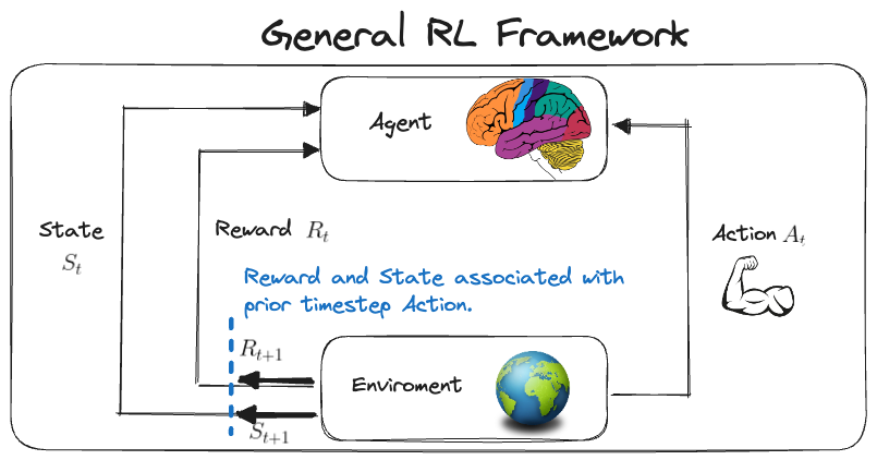
To understand this it’s worthwhile recapping the basics of RL. At it’s core RL can be thought of as a subset of ML which focuses on the problem of teaching a system (agent) how to behave (action) based on it’s enviroment (states) and work towards being successful in that enviroment (rewards). Diagramatically this would look something like below.
Teaching the system itself can be thought of as the trying to learn the optimal policy \(\pi^{*}\) which maximises the cumulative reward over time. This follows from the reward hypothesis which states that the all goals can be formulated as maximizing rewards over time.
Various methods exist for trying to find the optimal policy but broadly fall into two classes.
- Value based
- This works by learning a value function which you then can use to create a policy ontop of (such as the greedy epsilon policy which just takes the actions which maximize the value function).
- A value function can be formalised as \(v_{\pi} (s) = \mathbb{E}_{\pi}[G_{t} \vert S_{t} = s]\) where \(G_{t} = \sum_{k = 0}^{\infty} \gamma^{k} R_{t+k+1}\) represents the expected discounted return.
- The epsilon greedy policy can be thought of as a quasi-deterministic policy taking the form \(\pi(s) = \mathop{argmax}\limits_a Q^{*}(s, a)\).
- Policy based
- This works by approximating the policy directly either deterministically or stochastically. Deterministically would look like $a = \pi(s)$ and stochastically like \(\pi_{\theta}(a \vert s) = \mathbb{P}[A \vert s ; \theta]\) where the policy is just a probability distribution over the possible actions given a state.
- An objective function \(J(\theta)\) can then be used to represent the expected cumulative reward and so you can find the values of \(\theta\) which maximize this function.
Policy-gradient methods can be thought of as a subclass of the policy-based methods where the optimal policy \(\pi^{*}\) is directly modeled and the parameters of the objective function are optimized directly using the method of gradient ascent. Standard policy-based methods instead optimize the parameters indirectly by maximizing the local approximations with other techniques (hill climbing, simulated annealing or evolution strategies).
What are the steps to Policy gradient methods?
- Initialization:
- Initialize the policy \(\pi(a \vert s; \theta)\) with parameters \(\theta\).
- Data Collection:
- Use the current policy \(\pi(a \vert s; \theta)\) to collect trajectories by interacting with the environment. A trajectory \(\tau\) is a sequence of state-action-rewards \([s_0, a_0, r_0, s_1, a_1, r_1, \ldots]\).
- Objective Function:
- The objective is to maximize the expected return \(J(\theta)\) from the start state \(s_0\): \(J(\theta) = \mathbb{E}_{\tau \sim \pi(a|s; \theta)} \left[ R(\tau) \right]\) where \(R(\tau)\) is the total reward along a trajectory \(\tau\).
- Gradient Estimation:
- Calculate the gradient of the objective function with respect to the policy parameters $\theta$. The vanilla policy gradient is usually calculated as: \(\nabla J(\theta) = \mathbb{E}_{\tau \sim \pi(a|s; \theta)} \left[ \sum_{t=0}^{T} \nabla \log \pi(a_t|s_t; \theta) \cdot R(\tau) \right]\) where \(R(\tau)\) is the future discounted reward from time \(t\).
- Policy Update:
- Update the policy parameters $\theta$ in the direction that maximizes \(J(\theta)\): \(\theta \leftarrow \theta + \alpha \nabla J(\theta)\) where \(\alpha\) is the learning rate.
- Loop:
- Repeat steps 2-5 until convergence or a stopping criterion is met.
Variants and Enhancements
- Reward Shaping: Adjusting the reward function to make the learning process more efficient.
- Baseline Subtraction: To reduce variance in the gradient estimates, a baseline (often the value function $V(s)$) is subtracted from the rewards.
- Advanced Policy Gradients: Algorithms like Trust Region Policy Optimization (TRPO) and Proximal Policy Optimization (PPO) make more sophisticated updates to the policy.
- Actor-Critic Methods: These use a value function (the critic) to improve the policy (the actor).
- Exploration Strategies: Methods like entropy regularization encourage the policy to explore more.
Understanding the objective
Formally the objective function can be written as:
\[\begin{alignat*}{2} J(\theta) &= \mathbb{E}_{\tau \sim \pi_\theta}[R(\tau)] \quad && \scriptstyle{\text{; Definition of objective function being expected return.}} \\ &= \mathbb{E}_{\tau \sim \pi_\theta}[r_{t+1} + \gamma r_{t+2} + \gamma^{2} r_{t+3} +...+ \gamma^{n-1} r_{t+n}] \quad && \scriptstyle{\text{; Cumulative reward with discount factor } \gamma}\\ &= \sum_{\tau} P (\tau; \theta) R(\tau) \quad && \scriptstyle{\text{; Expectation being like a weighted average.}} \\ &= \sum_{\tau} {\color{red}{\prod_{t=0}^{n} P(s_{t+1} \vert s_{t}, a_{t})\pi_{\theta}(a_{t} \vert s_{t})}} R(\tau) \quad && \scriptstyle{\text{; Probability of a trajectory expansion}} \\ \end{alignat*}\]Deriving the policy gradient
Now having touched on what the objective is we outline some of the mathematical steps to actually compute the gradient of our objective below. The method we are showcasing utilises the Monte Carlo Reinforce algorithm for this.
Note: Formally the Policy Gradient Theorem states that $$ \nabla_\theta J(\theta) = \mathbb{E}_{\tau \sim \pi_\theta}[\nabla_\theta \log \pi_\theta (a_t \vert s_t) R(\tau)] $$ which is what we go on to show below. More details on how this works can be found here.\[\begin{alignat*}{2} \nabla_\theta J(\theta) &= \nabla_\theta \sum_{\tau} P(\tau; \theta) R(\tau) \quad && \scriptstyle{\text{; Starting definition of } J(\theta).} \\ &= {\color{red}{ \sum_{\tau} \nabla_\theta}} P(\tau; \theta) R(\tau) \quad && \scriptstyle{\text{; Gradient of sum as sum of gradients.}} \\ &= \sum_{\tau} {\color{red}{\frac{P(\tau; \theta)}{P(\tau; \theta)}}} \nabla_\theta P(\tau; \theta) R(\tau) \quad && \scriptstyle{\text{; Multiply and divide by } P(\tau; \theta).} \\ &= \sum_{\tau} P(\tau; \theta) {\color{red}{\nabla_\theta \log P(\tau; \theta)}} R(\tau) \quad && \scriptstyle{\text{; Apply log-derivative trick.}} \\ &= \mathbb{E}_{\tau \sim \pi_\theta}[\nabla_\theta \log \pi_\theta (a_t \vert s_t) R(\tau)] \quad && \scriptstyle{\text{; Result from the policy gradient theorem}} \\ &\approx {{\color{red}{\frac{1}{m} \sum_{i=1}^{m}}}} \nabla_\theta \log P(\tau^{(i)}; \theta) R(\tau^{(i)}) \quad && \scriptstyle{\text{; Estimate gradient with samples.}} \\ &\approx \hat{g} = \frac{1}{m} \sum_{i=1}^{m} \sum_{t=0}^{H} \nabla_\theta \log \pi_\theta(a_t^{(i)} | s_t^{(i)}) R(\tau^{(i)}) \quad && \scriptstyle{\text{; Final formula for policy gradient (using sampling).}} \end{alignat*}\]
Where you can expand the derivative of the logarithm as follows:
\[\begin{align*} \nabla_\theta \log P(\tau^{(i)}; \theta) &= \nabla_\theta \left[ \log \mu(s_0) + \sum_{t=0}^{H} \log P(s_{t+1}^{(i)} | s_t^{(i)}, a_t^{(i)}) + \sum_{t=0}^{H} \log \pi_\theta(a_t^{(i)} | s_t^{(i)}) \right]\\ &= \sum_{t=0}^{H} \nabla_\theta \log \pi_\theta(a_t^{(i)} | s_t^{(i)}) \quad \scriptstyle{\text{; Simplify gradient terms, } \mu(s_0) \text{ and } P(s_{t+1}^{(i)} | s_t^{(i)}, a_t^{(i)}) \text{ independent of } \theta} \end{align*}\]This is nice since we don’t need to deal with the MDP state transition dynamics since they don’t depend on \(\theta\).
Now it’s worth noting we have estimated the gradient by using the sample mean since it is formulated as an expectation (remember the sample mean is an unbiased estimator of the true population mean i.e \(\mathbb{E}(\bar{X}) = \mu\)). This sample mean is calculated over some set of trajectories \(\mathcal{D} = \{\tau_{i}\}_{i=1,...,m}\).