Table of Contents
- Introduction
- Multi-Armed Bandits Explained
- Algorithms and Techniques
- Application to Recommendation Models
- Future Directions
- Conclusions
Introduction
When you have an app or website one of your goals is to get people to engage with what you are creating, whether it be a product, service or something in between.
Recommendation systems play a crucial role in helping businesses attract, engage, and retain customers. However, the effectiveness of these systems largely depends on the accurate assignment of customers to the most suitable recommendation models. This is where multi-armed bandit algorithms come into play. In this blog post, we will explore how aligning multi-armed bandits for dynamic customer allocation can significantly optimize the performance of recommendation models.
Multi-Armed Bandits Explained
For historical context the term Bandit comes from the slot machines present in casinos, they were coined bandit since they ended up “stealing your money” just like a bandit would. Multi-Armed comes from fact people used to pull the levers (arms) of many slot machines at once.

Defintions
Lots of deep theory exists in this space but from a practical perspective having a basic grasp on some defintions is more than enough to begin working with these algorithms.
- Bandit specific
- The Multi-Armed Bandit Problem essentially is the problem of not knowing what the optimal decision to make is when faced with multiple options (“arms”).
- The process by which you can attempt solve these problems is to understand the specific context and then apply Multi-Armed Bandit Algorithms which are purposefully designed to tackle these problems.
- Reward just refers to the payoff or return recieved after selecting a particular action or arm of the multi-armed-bandit.
- Each arm of the bandit algorithm is associated with a reward distribution which tells you the likliehood of recieving a reward on any given round. When a given arm is pulled the reward recieved can be thought of as a realisation of this distribution.
- This distribution typically is unknown to the entity pulling the arms.
- The goal is to maximize the reward over a series of trials (arm pullings) while minimizing the regret, which is the difference between the reward recieved from an arm pull and the maximum reward that you would recieve if you always had chosen the best arm.
- Just like in RL the reward hypothesis can be used to assert that all goals can be thought of as a maximization of cumulative reward.
- The rewards themselves are stochastic in nature, meaning that they are randomly dertermined by the underlying probability distribution.
- This randomness introduces uncertainty and complexity into the decision making process as you must balance the tradeoff between exploring new arms to gather more information about their reward distributions (exploration) and exploiting known arms that have shown a high rewards in the past (exploitation). This is known as the exploration-exploitation trade-off problem.
- Some problem forumlations might have rewards that are context dependent where the reward distributions change based on external or contextual information available at the time of making a decision. This could add an additional strategic layer to the problem as the optimal action may vary with changes in the context.
- The Multi-Armed Bandit Problem essentially is the problem of not knowing what the optimal decision to make is when faced with multiple options (“arms”).
- Business specific
- An episode refers to the duration of time which a given customer stays assigned to the same bandit after which they are reallocated based on some process.
- When applying customer allocations a standard way is by staggering.
- The best way to think about it is as follows:
- Take the full customer base.
- Divide them into groups dependent on the length of the episodes (e.g if episode length = 28 days then group size = 1/28th of the base).
- Each day a single group gets allocated to an experiment.
- Therefore each day there would exist a group that is expiring from there previous episode and getting reallocated to another experiment.
- After a full episode length (e.g 28 days) all customers (across all groups) would have been through an entire episode and therefore would begin being reassigned (rolled over) to another episode.
- The best way to think about it is as follows:
Resources
Theory is well established in this space and as of now a few universally recognised reference materials exist along with a host of additional articles.
- Books
- Introduction to Multi-Armed Bandits; Aleksandrs Slivkins
- Universally recognised textbook, not super long but gives a good touch on most things.
- Bandit Algorithms; Tor Lattimore & Csaba Szepesvari
- Universally recognised reference book, alot longer but provides good technical grounding on the topic.
- Introduction to Multi-Armed Bandits; Aleksandrs Slivkins
- Lecture Material
- Online Learning and Multi-Armed Bandits Oxford
- Provides some links to prerequisite materials which is nice.
- Online Probability Summary Book
- Useful to brush up on Beta & Gamma distributions in particular.
- Online Learning and Multi-Armed Bandits Oxford
- Articles
- Introduction to Thompson Sampling: the Bernoulli bandit
- Good intro with particularily nice visualations to help internalise the bandit learning process.
- Introduction to Thompson Sampling: the Bernoulli bandit
Algorithms and Techniques
Plenty of algorithms and variants of them exist, we’ll touch on the three more common ones.
ε-Greedy
Pros:
- Simplicity: Easier to implement and understand in terms of how it implements the trae-off between exploration and exploitation.
Cons:
- Inefficient Exploration: Randomly explores at a fixed rate (set by \(\epsilon\)). Intuitively you should explore more initially to gain data and overtime once you have gathered more data you should exploit however in this case depending on your \(\epsilon\) you might not explore enough initially and not exploit enough later on.
- Flexibility: You’d want to choose $\epsilon$ based on the context of the problem but tuning it to find the right value might not be easy.
- Sub-optimal Decisioning: Due to constant exploration rate $\epsilon$ converging to the optimal bandit might take longer.
ε-Greedy Algorithm
    import numpy as np
    # e-greedy policy
    class eGreedyPolicy:

        def __init__(self, epsilon):
            """
            Initialize the eGreedyPolicy with a given epsilon value.

            Parameters
            ----------
            epsilon : float
                The probability of choosing a random action instead of the greedy action.
            """
            self.epsilon = epsilon

        def choose_bandit(self, k_array, reward_array, n_bandits):
            """
            Choose a bandit to pull based on the epsilon-greedy policy.

            Parameters
            ----------
            k_array : numpy.ndarray
                A 2D array where each row corresponds to a bandit and each column corresponds to the number of times a particular action has been taken.
            reward_array : numpy.ndarray
                A 2D array where each row corresponds to a bandit and each column corresponds to the rewards received for a particular action.
            n_bandits : int
                The number of bandits.

            Returns
            -------
            int
                The index of the chosen bandit.
            """
            # Successes and total draws
            success_count = reward_array.sum(axis=1)
            total_count = k_array.sum(axis=1)

            # Ratio of successes vs total
            success_ratio = success_count / total_count

            # Choosing best greedy action or random depending on epsilon probability
            if np.random.random() < self.epsilon:
                # Returning random action, excluding best
                return np.random.choice(np.delete(list(range(n_bandits)), np.argmax(success_ratio)))
            else:
                # Returning best greedy action
                return np.argmax(success_ratio)
Upper Confidence Bound (UCB)
Pros:
- Incorporating uncertainty: Instead of random exploration of bandits at a constant rate the exploration is embedded into the measure the algorithm is maximising by weighting with the frequency that the particular bandit in question has been assigned up until that point. By adding the extra square root term it upweights things which haven’t been seen as much, making it a better explorer than ε-greedy.
- Higher average reward: UCB doesn’t randomly explore and often achieves a higher average reward compared to ε-greedy since the additional term means more exploration earlier on (less reward) but way less for later rounds (more reward) causing the average to be better more often than not down the stretch. This also fits more closely with our intuition.
Cons:
- Complexity: It is more complex to implement and understand compared to ε-greedy.
- Computational Overhead: Since the algorithm requires calculating an additional confidence bound it can be a little more demanding than ε-greedy.
- Initial Exploration: Due to weighted exploration it may initially explore sub-optimal bandits more frequently meaning higher initial regret.
UCB Algorithm
    import numpy as np

    # UCB policy
    class UCBPolicy:

        def __init__(self):
            """
            Initialize the UCBPolicy.

            This constructor does not require any parameters.
            """
            pass

        def choose_bandit(self, k_array, reward_array, n_bandits):
            """
            Choose a bandit to pull based on the Upper Confidence Bound (UCB) policy.

            Parameters
            ----------
            k_array : numpy.ndarray
                A 2D array where each row corresponds to a bandit and each column corresponds to the number of times a particular action has been taken.
            reward_array : numpy.ndarray
                A 2D array where each row corresponds to a bandit and each column corresponds to the rewards received for a particular action.
            n_bandits : int
                The number of bandits.

            Returns
            -------
            int
                The index of the chosen bandit.
            """
            # Successes and total draws
            success_count = reward_array.sum(axis=1)
            total_count = k_array.sum(axis=1)

            # Ratio of successes vs total
            success_ratio = success_count / total_count

            # Computing square root term
            sqrt_term = np.sqrt(2 * np.log(np.sum(total_count)) / total_count)

            # Returning best greedy action
            return np.argmax(success_ratio + sqrt_term)
Thompson Sampling
Pros:
- Optimal Uncertainty Handling: Uses a Bayesian approach to model uncertainty, this is more sophisticated and has been shown to be empirically better than the other methods.
- More Adaptive: The exploration leverages the idea of sampling from posterior distributions which is a better representation than trying to either completely randomly explore (case of greedy) or altering the update measure (case of UCB). This leads to more efficient exploration and exploitation.
- Better Performance: It has been shown to outperform other algos in terms of cumulative reward across rounds.
Cons:
- Complexity: It is more complex to implement and understand compared to the other techniques.
- Computational Cost: Since the algorithm requires sampling and keeping track of the entire posterior distribution it can be costly especially if you have lots of bandits and rounds.
- Parameter Sensitive: It can be parameter sensitive in the sense that your choice on prior distributions.
Thompson Sampling Algorithm
    import numpy as np

    class TSPolicy:
        """
        Implements the Thompson Sampling policy for the Multi-Armed Bandit problem.

        Thompson Sampling is a probabilistic method that balances the exploration-exploitation trade-off by choosing actions based on the probability of them being optimal. This implementation assumes a Bernoulli bandit model where rewards are binary.

        Attributes
        ----------
        buffer_size : int
            The size of the buffer used to limit the history of rewards and actions considered. This is particularly useful for non-stationary bandits where the reward distributions change over time.

        Methods
        -------
        choose_bandit(k_array, reward_array, n_bandits)
            Chooses a bandit to play based on the Thompson Sampling algorithm.
        """

        def __init__(self, buffer_size):
            """
            Initializes the TSPolicy with a specified buffer size.

            Parameters
            ----------
            buffer_size : int
                The size of the buffer to limit the history of rewards and actions. A larger buffer size allows for more historical data to be considered, while a smaller size makes the policy adapt faster to changes in the reward distributions.
            """
            self.buffer_size = buffer_size

        def choose_bandit(self, k_array, reward_array, n_bandits):
            """
            Chooses a bandit to play based on the Thompson Sampling algorithm.

            This method calculates the posterior distribution of the success probability for each bandit based on the history of actions and rewards. It then samples from these distributions and chooses the bandit with the highest sample.

            Parameters
            ----------
            k_array : numpy.ndarray
                A 2D array where each row corresponds to a bandit and each column corresponds to the number of times a particular action has been taken. The shape of `k_array` is (n_bandits, n_actions).
            reward_array : numpy.ndarray
                A 2D array where each row corresponds to a bandit and each column corresponds to the rewards received for a particular action. The shape of `reward_array` is (n_bandits, n_actions).
            n_bandits : int
                The number of bandits.

            Returns
            -------
            int
                The index of the chosen bandit.
            """
            # Limiting the size of the buffer
            reward_array = reward_array[:, :k_array.sum(axis=1)][:, -self.buffer_size:]
            success_count = reward_array.sum(axis=1)
            failure_count = k_array.sum(axis=1) - success_count

            # Drawing a sample from each bandit distribution
            samples_list = [np.random.beta(1 + success_count[bandit_id], 1 + failure_count[bandit_id]) for bandit_id in range(n_bandits)]

            # Returning bandit with the best sample
            return np.argmax(samples_list)
Application to Recommendation Models
In the context of recommendation systems, multi-armed bandits can be applied to dynamically allocate customers to different recommendation models. Each recommendation model represents an “arm,” and the goal is to assign customers to the model that is most likely to provide them with relevant and satisfying recommendations. By using multi-armed bandit algorithms, the system can continuously learn and adapt its customer assignment strategy based on the observed performance of each recommendation model.
The better the performance the more assignments the arm will get and vice a versa.
Below I will share some of the core steps along with considerations you can take in order to apply bandit algorithms to your data. Specifically I’ll be showcasing the application of the Thompson Sampling algorithm
Defining our data
You need data for training your bandit algorithm as well as choosing the customers you want to perform assignments for. For demo purposes I’ll simultate some random data but in practice you’d want to create your dataset given your data sources. This most likely would require using some SQL dilect to transform your source data into something usable.
The key fields required:
- customer_id : int Some unique identifier for a customer, you can use multiple fields in practice to define a unique customer if a single id doesn’t exist.
- bandit_name : str The bandit that the given customer has been assigned too.
- reward : int Some reward corresponding to the performance of the customer, we will consider discrete reward her which could correpond to whether the customer clicked or engaged while being recommended content from the given bandit.
The training data typically would be some time back while the scoring would be based on the most recent events.
training_data = generate_fictitious_data(num_rows=10_000, customer_id_start=1)
assignment_data = generate_fictitious_data(num_rows=5000, customer_id_start=10_001)
generate_fictitious_data function
    def generate_fictitious_data(num_rows=5000, customer_id_start=1):
        """
        Generate a pandas DataFrame with fictitious data containing customer_id, bandit_name, and reward.

        Parameters
        ----------
        num_rows : int
            Number of rows in the DataFrame. Default is 5000.
        customer_id_start : int, optional
            Starting id for the customer_id. Default is 1.

        Returns
        -------
        df : pd.DataFrame
            DataFrame containing the generated data.
        """
        # Generate customer_id as unique numbers
        customer_ids = list(range(customer_id_start, customer_id_start + num_rows))

        # Generate bandit_name as random choices from 'A', 'B', 'C'
        bandit_names = [random.choice(['A', 'B', 'C']) for _ in range(num_rows)]

        # Generate reward as random binary values (0 or 1)
        rewards = [random.choice([0, 1]) for _ in range(num_rows)]

        # Create a dictionary with the generated data
        data = {
            'customer_id': customer_ids,
            'bandit_name': bandit_names,
            'reward': rewards
        }

        # Create a DataFrame from the dictionary
        df = pd.DataFrame(data)

        return df
Training our bandit
- High level steps:
- Setup a dataset that can store our bandit parameters.
- Take these parameters and initialise our Multi-Armed (Thompson Sampling) bandit algo with them.
- Feed in our historic training dataset and use it to update our Multi-Armed bandit model.
- Update (overwrite) our stored bandit parameters with the final parameters after training.
- We can also add in some visualisations too.
- Visualise the posterior distributions for each bandit after training to gauge the models understanding.
Initialise key constants
episode_length = 28
bandit_names = ['A', 'B', 'C']
Create a bandit parameter dataset
You’ll want to have someplace to store your bandit parameters since over time these will change and you’d need to use the latest parameters during assignment. Here I have decided to create a dataframe to hold these but for a real production system you could use some data store.
bandit_parameters = create_bandit_parameters_dataframe(bandit_names)
bandit_parameters.head()
create_bandit_parameters_dataframe function
    def create_bandit_parameters_dataframe(bandit_names):
        """
        Creates a DataFrame to store bandit parameters.

        Parameters
        ----------
        bandit_names : list
            The names of the bandits.

        Returns
        -------
        pd.DataFrame
            The created DataFrame with columns for bandit name, alpha, beta, and last_updated.
        """
        return pd.DataFrame({
            'bandit_name': bandit_names,
            'alpha': [1] * len(bandit_names),
            'beta': [1] * len(bandit_names),
            'last_updated': [datetime.now()] * len(bandit_names)
        })
Train your bandit
We can now train our bandit by applying it to our historical training data, this allows the algorithm to learn upfront which bandit arm tends to give the most reward and so can these learnings can be put into good use when assigning customers.
ts, bandit_parameters = train_bandits(bandit_parameters,
                    training_data,
                    bandit_names)
bandit_parameters.head()
train_bandits functionality
    class ThompsonSampling:
    """
    Implements the Thompson Sampling algorithm for the Multi-Armed Bandit problem.

    Attributes
    ----------
    bandit_names : list
        The names of the bandits (arms).
    alpha : np.ndarray
        Array of alpha parameters (successes) for the Beta distribution of each bandit.
    beta : np.ndarray
        Array of beta parameters (failures) for the Beta distribution of each bandit.

    Methods
    -------
    choose_bandit()
        Chooses a bandit to play based on the Thompson Sampling algorithm.
    update(chosen_bandit, reward)
        Updates the parameters of the chosen bandit's Beta distribution based on the observed reward.
    """
    def __init__(self, bandit_names, alpha=None, beta=None):
        """
        Initialises the ThompsonSampling class with the specialised number of bandits.

        Parameters
        ----------
        n_bandits : int
            The number of bandits (arm).
        """

        self.bandit_names = bandit_names
        self.alpha = alpha if alpha is not None else {name: 1 for name in bandit_names}
        self.beta = beta if beta is not None else {name: 1 for name in bandit_names}

    def choose_bandit(self):
        """
        Chooses a bandit to play based on the Thompson Sampling algorithm.

        This method samples from the Beta distribution of each bandit and selects the bandit with the highest sample.

        Returns
        -------
        str
            The name of the chosen bandit.
        """

        expected_reward_samples = {name: beta.rvs(self.alpha[name], self.beta[name], size=1) for name in self.bandit_names}
        return max(expected_reward_samples, key=expected_reward_samples.get)

    def update(self, chosen_bandit, reward):
        """
        Updates the parameters of the chosen bandit's Beta distribution based on the observed reward.

        Parameters
        ----------
        chosen_bandit : str
            The name of the chosen bandit.
        reward : int
            The observed reward (1 for success, 0 for failure).
        """
        if reward:
            self.alpha[chosen_bandit] += 1
        else:
            self.beta[chosen_bandit] += 1

    def train_bandits(bandit_params_df, customer_data_df, bandit_names, limit=0):
        """
        Perform assignment of customers to bandits over a specified episode length using Thompson Sampling.

        Parameters
        ----------
        bandit_params_df : pd.DataFrame
            The DataFrame containing bandit parameters.
        customer_data_df : pd.DataFrame
            The DataFrame containing customer data.
        bandit_names : list
            The names of bandits (arms).
        limit : int, optional
            The limit on the number of customers to consider for training. Default is 0 (no limit).

        Returns
        -------
        ts : ThompsonSampling
            The trained ThompsonSampling instance.
        """
        # Retrieve bandit parameters from DataFrame
        bandit_params = get_bandit_parameters_from_dataframe(bandit_params_df, bandit_names)
        alpha = {name: bandit_params[name][0] for name in bandit_names}
        beta = {name: bandit_params[name][1] for name in bandit_names}

        ts = ThompsonSampling(bandit_names, alpha, beta)

        if limit > 0:
            customer_data_df = customer_data_df.sample(n=limit)

        for _, row in customer_data_df.iterrows():
            ts.update(row['bandit_name'], row['reward'])

        # Update the bandit parameters in DataFrame
        for bandit_name in bandit_names:
            update_bandit_parameters_in_dataframe(bandit_params_df, bandit_name, ts.alpha[bandit_name], ts.beta[bandit_name])

        return ts, bandit_params_df

    def get_bandit_parameters_from_dataframe(bandit_params_df, bandit_names):
        """
        Retrieves the alpha and beta parameters for each bandit from the DataFrame.

        Parameters
        ----------
        bandit_params_df : pd.DataFrame
            The DataFrame containing bandit parameters.
        bandit_names : list
            The names of the bandits.

        Returns
        -------
        dict
            A dictionary with bandit names as keys and (alpha, beta) tuples as values.
        """
        bandit_params = {}
        for name in bandit_names:
            row = bandit_params_df[bandit_params_df['bandit_name'] == name]
            if not row.empty:
                bandit_params[name] = (row['alpha'].values[0], row['beta'].values[0])
            else:
                bandit_params[name] = (1, 1)
        return bandit_params

    def update_bandit_parameters_in_dataframe(bandit_params_df, bandit_name, alpha, beta):
        """
        Updates the alpha and beta parameters for a specific bandit in the DataFrame.

        Parameters
        ----------
        bandit_params_df : pd.DataFrame
            The DataFrame containing bandit parameters.
        bandit_name : str
            The name of the bandit.
        alpha : float
            The updated alpha parameter.
        beta : float
            The updated beta parameter.
        """
        if bandit_name in bandit_params_df['bandit_name'].values:
            bandit_params_df.loc[bandit_params_df['bandit_name'] == bandit_name, ['alpha', 'beta', 'last_updated']] = [alpha, beta, datetime.now()]
        else:
            new_row = pd.DataFrame({
                'bandit_name': [bandit_name],
                'alpha': [alpha],
                'beta': [beta],
                'last_updated': [datetime.now()]
            })
            bandit_params_df = pd.concat([bandit_params_df, new_row], ignore_index=True)
Visualise the posterior distributions
It’s useful to get a feel for exactly what the model has learned and this can be done by visualising the posterior distributions generated for each of the bandits limbs. If the distributions are heavily peaked with differing expected values this can mean the model will exploit more since it’s more likely that a large reward will come from the distribution with the higher expected value (more divergence implies less overlap therefore unlikely to get anything from the low distributions).
plot_posterior_distributions(ts)
plot_posterior_distributions function
    def plot_posterior_distributions(ts_instance, fig_size=(12,8)):
        """
        Plots the posterior Beta distributions for each bandit in the ThompsonSampling instance.

        Parameters
        ----------
        ts_instance : ThompsonSampling
            An instance of the ThompsonSampling class.
        fig_size : tuple, optional
            A tuple representing the figure size (width, height).

        Returns
        -------
        None
            The function displays the plot and doesn't return anything.
        """

        n_bandits = len(ts_instance.bandit_names)
        n_rows = np.ceil(n_bandits / 2).astype(int)
        n_cols = 2

        fig, axes = plt.subplots(n_rows, n_cols, figsize=fig_size)
        if n_rows > 1:
            axes = axes.flatten()
        else:
            axes = [axes]

        for sub_plot, bandit_name in enumerate(ts_instance.bandit_names):
            a = ts_instance.alpha[bandit_name]
            b = ts_instance.beta[bandit_name]
            reward = np.linspace(0, 1, 100)
            y = beta.pdf(reward, a, b)
            peak_reward = reward[np.argmax(y)]

            axes[sub_plot].plot(reward, y, label=f"Beta({a}, {b})")
            axes[sub_plot].set_title(f"Posterior: {bandit_name} \n Success: {int(a)}, Failure: {int(b)}")
            axes[sub_plot].set_xlabel('Expected Reward')
            axes[sub_plot].axvline(x=peak_reward, color='red', linestyle=':', linewidth=2, label=f"'Average' Expected Reward: {peak_reward:.2f}")
            # axes[sub_plot].text(peak_reward, -1, f'(peak_reward:.2f)', ha='center', va='bottom', color='red')

            axes[sub_plot].legend()
            axes[sub_plot].grid(True)
            axes[sub_plot].set_facecolor('lightgrey')

        for j in range(sub_plot + 1, n_rows * n_cols):
            axes[j].axis('off')

        plt.tight_layout()
        plt.show()
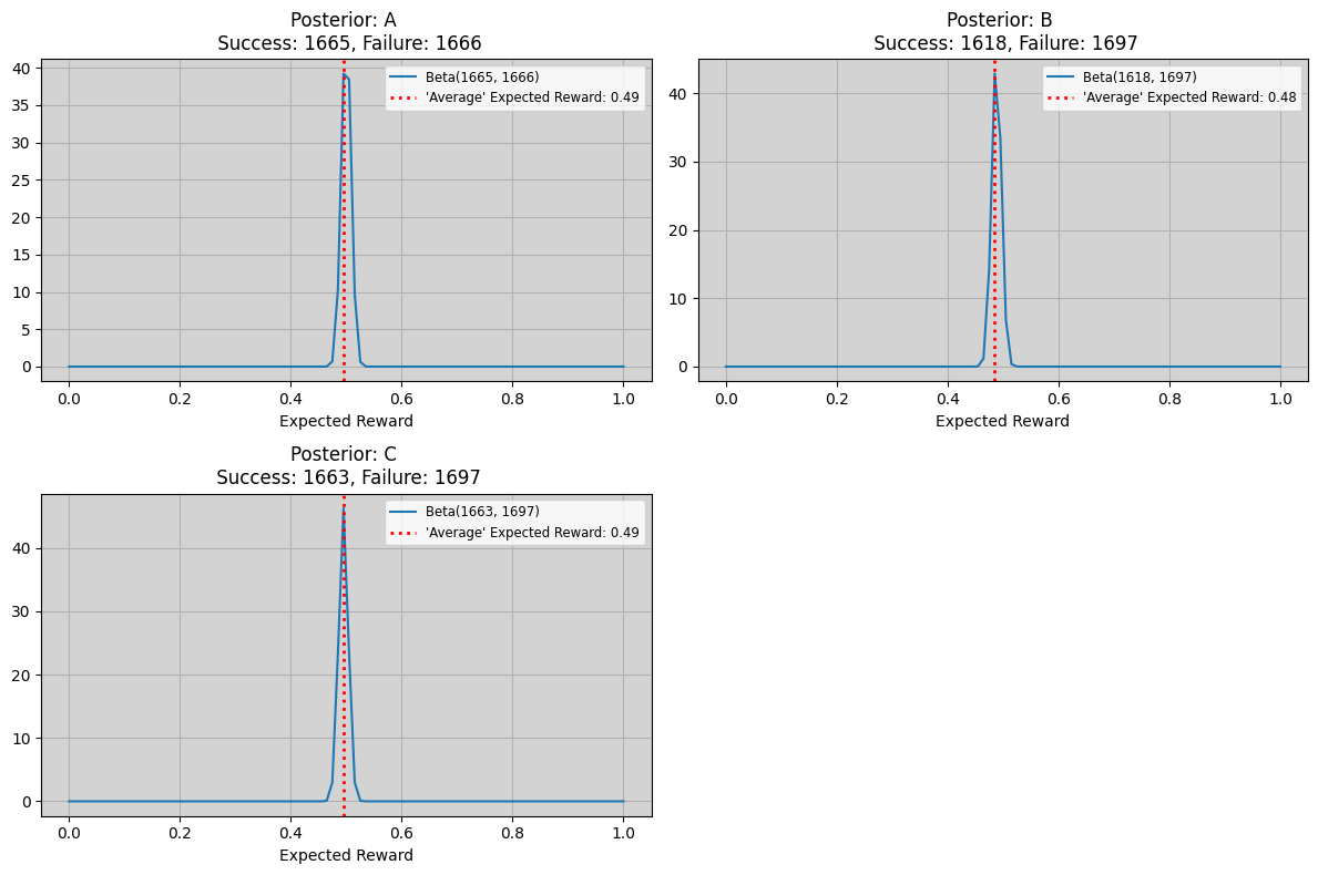
As you can see the distributions are fairly close togther and not divergent. This makes intuitive sense as it aligns with what we’d expect given the process used to construct our training dataset.
Performing customer assignment
- High level steps:
- Grab the customers that you want to allocate.
- Take the initially trained bandit algorithm and apply it to each customer making sure to update its parameters after each assignment.
- Make the assignments for all customers and store them alongside other metadata such as dates for the start and end of the assignment inside some data structure.
- Update our stored bandit parameters with the final values.
- We can also add some visualisations in too:
- Visualise the customer groups most recent reward distribution (based on the episode they are rolling out of).
- Visualise the final bandit allocation distributions.
Visualsing real reward distribution
plot_reward_distribution(assignment_data,
                               group_col="bandit_name",
                               reward_col="reward")
plot_reward_dsitrbution function
    def plot_reward_distribution(data, group_col, reward_col, fig_size=(12, 8)):
        """
        Plot the distribution of reward.

        Parameters
        ----------
        data : pd.DataFrame
            The input dataset containing customer ID, group column, reward and other fields.
        group_col : str
            The name of the column indicating the group for each customer.
        reward_col : str
            The name of the column containing the reward values.
        fig_size : tuple, optional
            The size of the figure (width, height) in inches. Default is (12, 8).

        Returns
        ------
        None
            The function displays the plot and does not return any value.
        """

        groups = data[group_col].unique()
        num_groups = len(groups)

        n_cols=2
        n_rows = (num_groups + n_cols - 1) // n_cols
        fig, axes = plt.subplots(nrows=n_rows, ncols=n_cols, figsize=fig_size)

        for i, group in enumerate(groups):
            # Calculate the row and column indices for the current subplot
            row_idx = i // n_cols
            col_idx = i % n_cols

            group_data = data[data[group_col] == group]
            reward_counts = group_data[reward_col].astype(int).value_counts()
            reward_counts = reward_counts.reindex([0, 1], fill_value=0)

            plot_data = pd.DataFrame({
                'Reward': reward_counts.index,
                'Count': reward_counts.to_numpy()
            })

            sns.barplot(x='Reward', y='Count', data=plot_data, ax=axes[row_idx, col_idx])
            axes[row_idx, col_idx].set_title(f'Group: {group}')
            axes[row_idx, col_idx].set_xlabel(f'Reward')
            axes[row_idx, col_idx].set_ylabel(f'Count')
            axes[row_idx, col_idx].set_ylim([0, data.shape[0]])
            axes[row_idx, col_idx].set_facecolor('lightgray')

        for bar in axes[row_idx, col_idx].patches:
            count = bar.get_height()
            axes[row_idx, col_idx].text(bar.get_x() + bar.get_width() / 2, bar.get_height(), str(int(count)), ha='center', va='bottom')

        plt.tight_layout()
        plt.show()

Performing Assignments
customer_assignments, bandit_parameters = assign_customers(bandit_parameters,
                       assignment_data,
                       bandit_names,
                       episode_length,
                       ts)
customer_assignments.head()
assign_customers function
    def assign_customers(bandit_params_df, customer_data_df, bandit_names, episode_length, ts, limit=0):
        """
        Perform assignment of customers to bandits over a specified episode length using Thompson Sampling.

        Parameters
        ----------
        bandit_params_df : pd.DataFrame
            The DataFrame containing bandit parameters.
        customer_data_df : pd.DataFrame
            The DataFrame containing customer data.
        bandit_names : list
            The names of the bandits.
        episode_length : int
            The length of the episode in days.
        ts : ThompsonSampling
            The trained ThompsonSampling instance.
        limit : int, optional
            The limit on the number of customers to assign. Default is 0 (no limit).

        Returns
        -------
        customer_assignments : pd.DataFrame
            A DataFrame containing each customer's ID, the assigned bandit, and the start and end dates of their episode.
        """
        assignments = []
        start_date = datetime.now()

        if limit > 0:
            customer_data_df = customer_data_df.sample(n=limit)

        # Perform assignment process
        for _, row in customer_data_df.iterrows():
            chosen_bandit = ts.choose_bandit()
            ts.update(row['bandit_name'], row['reward'])
            assignments.append({
                'customer_id': row['customer_id'],
                'bandit_name': chosen_bandit,
                'start_date': start_date,
                'end_date': start_date + timedelta(days=episode_length)
            })

        # Update the bandit parameters in DataFrame
        for bandit_name in bandit_names:
            update_bandit_parameters_in_dataframe(bandit_params_df, bandit_name, ts.alpha[bandit_name], ts.beta[bandit_name])

        customer_assignments = pd.DataFrame(assignments)

        return customer_assignments, bandit_params_df
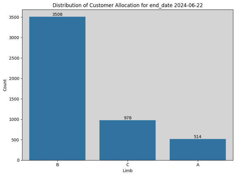
Visualising assignment distributions
plot_bandit_assignment_distributions(customer_assignments,
                                           "bandit_name",
                                           "end_date")
plot_bandit_assignment_distributions function
    def plot_bandit_assignment_distributions(data, bandit_col, group_date, fig_size=(8, 6)):
        """
        Plot the counts of assignments made by the bandit algorithm.

        Parameters
        ----------
        data : pd.DataFrame
            The input dataset containing the bandit assignments.
        bandit_col : str
            The name of the column to calculate the counts (bandit assignment col).
        group_date : str
            The name of the column containing the date (identifying a given group).
        fig_size : tuple, optional
            The size of the figure (width, height) in inches. Default is (8, 6).

        Returns
        -------
        None
            The function displays the plot and doesn't return anything.
        """

        column_counts = data[bandit_col].value_counts()
        group_name = f"{data[group_date].unique()[0].strftime('%Y-%m-%d')}"

        fig, ax = plt.subplots(figsize=fig_size)

        sns.barplot(x=column_counts.index, y=column_counts.to_numpy(), ax=ax)
        ax.set_title(f"Distribution of Customer Allocation for group end_date {group_name}")
        ax.set_xlabel('Limb')
        ax.set_ylabel('Count')
        ax.set_facecolor('lightgrey')

        for bar in ax.patches:
            count = bar.get_height()
            ax.text(bar.get_x() + bar.get_width() / 2, bar.get_height(), str(int(count)), ha='center', va='bottom')

        plt.tight_layout()
        plt.show()
Future Directions
Many ways to extend the work here, I have listed a few directions below:
- Handle continuous rewards
- At the moment the Thompson Sampling algorithm only applies for the discrete reward case.
- To adapt for continuous rewards things like the bayesian prior and update logic will need to be extended.
- Over aggresive assignment handling
- At the moment if you train on too much data your posterior distributions can become extremely peaked and divergent which can lead to almost always assigning to the most performant bandit.
- This might not always be desired espeically in a practical setting as you may want some variation to continue to monitor behaviour between the recommendation models.
- Some potential ways to adapt are:
- Sliding Window: This would cap the total amount of rewards that a given bandit could recieve thereby limiting how peaked the distributions can become. Challenge might be optimizing the threshold for the problem.
- Contextual reward handling
- In alot of real world cases the reward can vary over time due to a variety of factors including the context.
- To handle this you’d want to adapt the “Vanilla MAB” approach for more of a “Contextual MAB” approach.
- Plently of resources touch on it, this somewhat recent lecture at the PyData conference might be a nice place to start.
SlidingWindow Approach
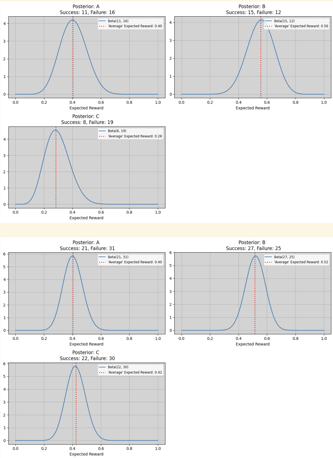
When using a Sliding Window approach it might be necessary to restrict how peaked the posterior distributions get. In our case this is necessary since we want to limit the aggressiveness of the final limb assignments and if we don’t restrict the window size then the resulting distributions will end up diverging (minimal overlap) and therefore resulting samples would almost always be chosen from the distribution with the highest average expected reward.
sliding window algorithm
    class SlidingWindowThompsonSampling(ThompsonSampling):
        """
        Implements the Sliding Window functionality on our Thompson Sampling class.

        Attributes
        ----------
        bandit_names : list
            The names of the bandits (arms).
        alpha : np.ndarray
            Array of alpha parameters (successes) for the Beta distribution of each bandit.
        beta : np.ndarray
            Array of beta parameters (failures) for the Beta distribution of each bandit.
        window_size : int
            The size of the window (max number of rewards that can be used to build posterior distributions).
        rewards : list
            List of rewards (both a reward and no reward would add an element) for each of the bandits.

        Methods
        -------
        update(chosen_bandit, reward)
            Updates the parameters of the chosen bandit's Beta distribution based on the observed reward.
        """
        def __init__(self, bandit_names, window_size=1000, **kwargs):
            super().__init__(bandit_names, **kwargs)
            self.window_size = window_size
            self.rewards = {name: deque(maxlen=self.window_size) for name in bandit_names}

        def update(self, chosen_bandit, reward):
            # Selecting the reward deque of the bandit we are updating
            rewards_deque = self.rewards[chosen_bandit]

            # Updating reward deque using the reward we have just observed
            rewards_deque.append(reward)

            # Checking to see if the reward deque is above our desired cutoff window size.
            # Making smaller if so.
            # if len(rewards_deque) > self.window_size:
            #     rewards_deque.popleft()

            # Calculating our new successes and failures
            reward_sum = int(sum(rewards_deque))
            new_alpha = 1 + reward_sum
            new_beta = 1 + (len(rewards_deque) - reward_sum)

            # Updating our alpha and beta parameters of the updated bandit with the latest info.
            self.alpha[chosen_bandit] = new_alpha
            self.beta[chosen_bandit] = new_beta
There are several different approaches to handle this problem as listed below:
- Empirical Tuning
- Steps:
- Specify your desired resultant assignment proportions along with an acceptable threshold deviation value away from these proportions.
- Looping over some predefined window sizes (smallest to largest).
- Each window size instantiates its own SlidingWindowThompsonSampling algorithm and is trained on some specified historical training dataset.
- Make assignments on a historical assignment dataset.
- Evaluating each window size based on how close resulting assignments are to desired proportions are on the historical assignment dataset.
- Choose the largest possible window size (exploitation) which still yields an acceptable level of closeness from the desired proportions.
- This can help the distributions from becoming too peaked by training historically on data and then measuring assignments on some other data and ensuring the proportions of assignments are close enough to what we desired. This way the window size has balanced exploiting known top-performing bandits and exploration by ensuring assignments are diverse.
- Steps:
- Adaptive Windowing
- Steps:
- Change the window size depending on the changes within the underlying data stream.
- Measure the mean between difference sub windows of your rewards for each bandit.
- If a difference is present between the mean reward of two sub-windows by some delta of the standard deviation then we say a difference is present.
- Upon each update of the distributions reward a calculation is done to see if a change is detected on any sub window.
- If yes then the window size is halved to allow the distribution to pick up the change more easily.
- If no then the window size is just incremented to make it a little higher.
- Change the window size depending on the changes within the underlying data stream.
- This can help the distributions from becoming too peaked by constantly adapting the window sizes over time as updates are made and ensures this is done dynamically.
- Steps:
Empircal Tuning of Window size
Here is a brief look at what the output of the empirical tuning process would look like. You’ll want to insure you use appropriate training and assignment datasets but the general process should look similar:
# Define parameters
bandit_names = ['A', 'B', 'C']
window_sizes = [25, 50, 75, 100, 500, 1000]
desired_proportions = {
    'A': 0.33,
    'B': 0.33,
    'C': 0.34
}
difference_threshold = 0.10

# Generate training and assignment data
training_data = generate_fictitious_data(num_rows=10_000, customer_id_start=1)
assignment_data = generate_fictitious_data(num_rows=5_000, customer_id_start=10_001)

# Call the empirical_window_size_tuning function
best_window_size, best_assignments = empirical_window_size_tuning(
    bandit_names=bandit_names,
    window_sizes=window_sizes,
    training_data=training_data,
    assignment_data=assignment_data,
    desired_proportions=desired_proportions,
    difference_threshold=difference_threshold
)
empirical tuning functionality
    def evaluate_window_size(bandit_names, window_size, training_data, assignment_data, desired_proportions, difference_threshold=0.3):
        """
        Parameters
        ----------
        bandit_names : list
            List of the bandit names to use to instantiate our ThompsonSampling instance.
        window_size : int
            The size of the window we want to use for our ThompsonSampling instance.
        training_data : pd.DataFrame
            Data used to update our bandits model parameters on.
        assignment_data : pd.DataFrame
            Data used to make assignments and measure assignment distribution on.
        desired_proportions : dict
            Dictionary containing the limb names and our desired proportions.
        difference_threshold : float, optional
            Threshold specifying the max acceptable difference from our threshold.

        Returns
        -------
        final_assignments : pd.DataFrame
            DataFrame containing the assignments on the assignment dataset.
        None
            If the actual proportions don't align with the desired proportions across any of the limbs within our specified difference threshold.
        """
        # Instantiate our Thompson Sampling class
        ts = SlidingWindowThompsonSampling(bandit_names, window_size=window_size)

        # Update the parameters of the instance using the training data.
        for _, row in training_data.iterrows():
            ts.update(row['bandit_name'], row['reward'])

        # Plotting trained distribution
        plot_posterior_distributions(ts)

        # Perform assignments using the assignment data
        assignments = []
        for _, row in assignment_data.iterrows():
            chosen_bandit = ts.choose_bandit()
            ts.update(chosen_bandit, row['reward'])
            assignments.append({
                'customer_id': row['customer_id'],
                'bandit_name': chosen_bandit,
            })

        final_assignments = pd.DataFrame(assignments)

        # Calculate the assignment proportions
        assignment_proportions = final_assignments['bandit_name'].value_counts(normalize=True).to_dict()

        for bandit_name, desired_proportion in desired_proportions.items():
            actual_proportion = assignment_proportions.get(bandit_name, 0)
            observed_difference = abs(actual_proportion - desired_proportion)

            if observed_difference > difference_threshold:
                print(f"Window Size: {window_size} failed with:")
                print(f"\tBandit Name: {bandit_name}, Actual Prop: {actual_proportion:.4f}, Desired Prop: {desired_proportion:.4f}, Difference: {observed_difference:.4f}, Threshold: {difference_threshold}")
                return None

        return final_assignments

    def empirical_window_size_tuning(bandit_names,
                                    window_sizes,
                                    desired_proportions,
                                    difference_threshold):
        """
        Parameters
        ----------
        bandit_names : list
            List of bandit names.
        window_sizes : list
            List of window sizes to evaluate.
        desired_proportions : dict
            Dictionary containing the limb names and our desired proportions.
        difference_threshold : float
            Threshold specifying the max acceptable difference from our threshold.

        Returns
        -------
        results : dict
            Dictionary containing the results for each window size.
        """
        results = {}

        # Generate training and assignment data
        training_data = generate_fictitious_data(num_rows=10_000, customer_id_start=1)
        assignment_data = generate_fictitious_data(num_rows=5_000, customer_id_start=10_001)

        for window_size in window_sizes:
            final_assignments = evaluate_window_size(
                bandit_names=bandit_names,
                window_size=window_size,
                training_data=training_data,
                assignment_data=assignment_data,
                desired_proportions=desired_proportions,
                difference_threshold=difference_threshold
            )

            if final_assignments is not None:
                results[window_size] = final_assignments
            else:
                results[window_size] = "Failed to meet desired proportions"

        return results
You can then take a quick look at the resulting best window size and go back and use this inside your prior code (when defining the window size to use when training your intial bandit model).
# Display the results
print(f"Best Window Size: {best_window_size}")
if best_assignments is not None:
    display(best_assignments.head())
else:
    print("No window size met the desired proportions within the specified threshold.")
Output:
Best Window Size: 25
customer_id	bandit_name
0	10001	C
1	10002	B
2	10003	B
3	10004	C
4	10005	A
If all things have gone well then when viewing the distribution of your assignments you should hopefully see resemblance to the proportions you specified at the beginning of tuning.
best_assignments['bandit_name'].value_counts(normalize=True)
In other words something like:
bandit_name
A    0.4206
C    0.3188
B    0.2606
Name: proportion, dtype: float64
Dynamic Adaption of Window size
Now I’ll leave this to the user to have a think about; I suspect a number of ways can be used to perform adaptive windowing. Below is a brief sketch out of one of those ways.
class AdaptiveSlidingWindowThompsonSampling(ThompsonSampling):
    """
    Implement an Adaptive Sliding Window functionality onto our Thompson Sampling class.

    Attributes
    ----------
    bandit_names : list
        The names of the bandits (arms).
    alpha : np.ndarray
        Array of alpha parameters (successes) for the Beta distribution of each bandit.
    beta : np.ndarray
        Array of beta parameters (failures) for the Beta distribution of each bandit.
    window_size : int
        The size of the window (max number of rewards that can be used to build posterior distributions).
    rewards : Dict[list]
        List of rewards (both a reward and no reward would add an element) for each of the bandits.
    adwin : Dict[ADWIN]
        An ADWIN class instance for each of the bandit names to monitor its reward and subsequently adjust window size to avoid it getting too peaked.

    Methods
    -------
    update(chosen_bandit, reward)
        Updates the parameters of the chosen bandit's Beta distribution based on the observed reward.
    """

    def __init__(self, bandit_names, initial_window_size=1000, delta=0.002, **kwargs):
        super().__init__(bandit_names, **kwargs)
        self.window_size = initial_window_size
        self.rewards = {name: deque() for name in bandit_names}
        self.adwin = {name: ADWIN(delta) for name in bandit_names}

    def update(self, chosen_bandit, reward):
        rewards_deque = self.rewards[chosen_bandit]
        adwin = self.adwin[chosen_bandit]

        rewards_deque.append(reward)
        adwin.add_element(reward)

        if adwin.detected_change():
            self.window_size = max(1, self.window_size // 2)  # Shrink window to make it more adaptive to observed change
        else:
            self.window_size = min(self.window_size * 2, 1000)  # Grow window to make estimates more stable

        if len(rewards_deque) > self.window_size:
            rewards_deque.popleft()

        reward_sum = int(sum(rewards_deque))
        new_alpha = 1 + reward_sum
        new_beta = 1 + (len(rewards_deque) - reward_sum)

        self.alpha[chosen_bandit] = new_alpha
        self.beta[chosen_bandit] = new_beta
Where the quantification of growth and shrinkage of the window is somewhat arbitrary (might be worth tweaking).
ADWIN functionality
    class ADWIN:
        """
        Define Adaptive Windowing functionality to detect whether incoming datastream shows a difference.

        Attributes
        ----------
        delta : float
            A parameter that controls the sensitivity of the change detection. Smaller values make the algorithm more sensitive to changes.
        width : int
            The current size of the window.
        total : int
            The sum of the total values in the window (positive reward).
        variance : float
            The sum of the squared values in the window.
        window : list
            A list that stores the data points in the current window.

        Methods
        -------
        add_element(value)
            Adds a new reward data point to the window and checks for changes between the given window sub_windows.
        detected_change()
            Returns the value of the `drift_detected` flag.
        """

        def __init__(self, delta=0.05):
            self.delta = delta
            self.width = 0
            self.total = 0
            self.variance = 0
            self.window = deque()
            self.drift_detected = False

        def add_element(self, value):
            self.window.append(value)
            self.width += 1
            self.total += value
            self.variance += value**2

            if self.width > 1:
                mean = self.total / self.width
                variance = (self.variance / self.width) - (mean**2)
                std_dev = np.sqrt(variance)

                for i in range(1, self.width):
                    sub_window_1 = list(self.window)[:i]
                    sub_window_2 = list(self.window)[i:]
                    mean_1 = np.mean(sub_window_1)
                    mean_2 = np.mean(sub_window_2)

                    if abs(mean_1 - mean_2) > self.delta * std_dev:
                        self.drift_detected = True
                        self.window = deque(sub_window_2)
                        self.width = len(self.window)
                        self.total = sum(self.window)
                        self.variance = sum([x**2 for x in self.window])
                        break
                    else:
                        self.drift_detected = False

        def detected_change(self):
            return self.drift_detected
Conclusions
With all this we come to the end, hopefully it’s been insightful and have got a peer into the purpose behind Multi-Armed Bandit problems and specifically how Thompson Sampling can be appled to the case of Customer Assignment and how it can be beneficial.