Table of Contents
- Introduction: The Dawn of Large Language Models
- The Mechanics of Large Language Models
- Evolution of Large Language Models
- Applications of Large Language Models
- Challenges and Limitations of Large Language Models
- Working with Large Language Models: A Practical Guide
- Conclusion: Reflection
- Reference Material & Further Reading
Introduction: The Dawn of Large Language Models
The term large language model has been thrown around alot recently, news outlets, YouTube videos, forum posts and even peoples personal blog sites 😅 but what actually is it? Well luckily for us it’s fairly intuitive from the name.
- “Large” refers to the fact the underlying models are trained on a vast quantities of data and have lots of parameters which make them up.
- These models are essentially neural networks under the hood and so have lots of weights which are tuned to make the model as good as possible.
- The deeper and wider these networks are the more weights they will contain which in turn relates to the fact that they are “large” quote on quote.
- “Language” references the fact that these models were specifically designed to work with language i.e natural language text data.
- They were trained with the objective of trying to understand in a general sense the patterns within text data.
- The hopes are that being trained with this language understanding would mean the model could perform well on narrow objectives such as content generation, translation, Q&A, sentiment analysis, information extraction etc.
- “Model” is relatively ambigous term which in this context can refer to a tangible thing which to some degree acts as a representation of the truth.
- Models in general are our (humans) way of representing reality using our scientific language (mathematics). A famous quote from George Box showcases this point “All models are wrong, but some are useful.”
- Models are useful to help progress our understanding of things (hopefully important things), allowing us to build ontop of others work objectively and make improvements overtime. John Tukey said it well that “An approximate answer to the right problem is worth a good deal more than an exact answer to an approximate problem.”
- Currently the best models utilise neural networks which were inspired by the human brain, essentially a mathematical soup of Linear Algebra sprinkled with non-linearities to model language.
Putting two and two together we can form a fairly concise defintion being that it’s a “large model (typically neural network based) which is trained on a bunch of language to gain general purpose language understanding in the hopes of being able to achieve good performance on language based tasks.”
The Mechanics of Large Language Models
Now, given the definition we have formed above it’s not hard to see that it doesn’t specify a particular model architecture. This is slightly counter-intuitive esspecially for those who would have heard LLMs in the context of applications like ChatGPT.
With this in mind here is a small list of various model architectures which could fall into the bucket of being classed as an LLM under certain condtions.
- Recurrent Neural Networks (RNNs):
- These models are designed to recognize patterns in sequences of data, such as text, genomes, handwriting, or the spoken word. They are called recurrent because they perform the same task for every element of a sequence, with the output being dependent on the previous computations.
- RNNs have a “memory” known as the hidden state which captures information about text across sequential postitions.
- Good examples of other RNN based architectures include LSTM (Long Short-Term Memory) and GRU (Gated Recurrent Units).
- Transformers:
- Transformers are a type of model that use self-attention mechanisms and are particularly effective for large-scale language tasks.
- They process input data in parallel (as opposed to sequentially in RNNs), making them more efficient for handling large datasets.
- The Transformer model forms the basis of many state-of-the-art models such as BERT (Bidirectional Encoder Representations from Transformers), GPT (Generative Pretrained Transformer), and T5 (Text-to-Text Transfer Transformer).
- Convolutional Neural Networks (CNNs) for Text:
- While CNNs are traditionally used for image processing, they can also be used for text analysis. In the context of language processing, CNNs can be used to detect local dependencies in sentences, and are often used for tasks like sentiment analysis and topic categorization.
- Hybrid Models:
- These models combine elements from different types of models. For example, the Transformer-RNN model combines a Transformer’s ability to capture global dependencies with an RNN’s capacity to model local, sequential dependencies.
Here is a view of what the RNN architecture looks like:
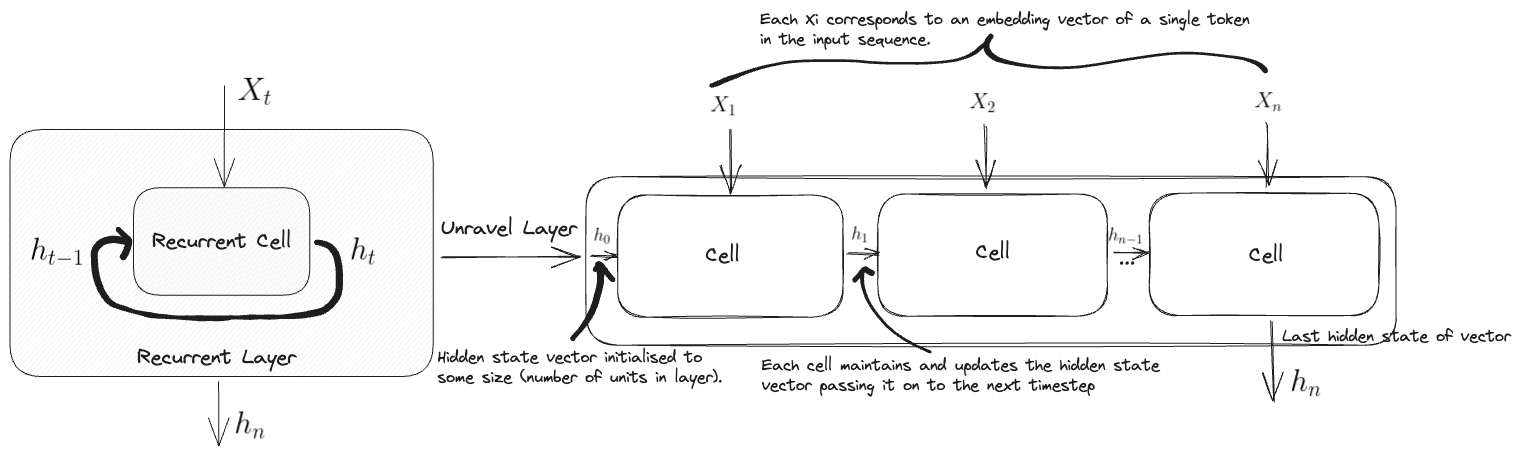
Where $X_t$ represents the input at a given timestep (imagine some sequential inputs $X_1, X_2,…X_n$), $h_{t-1}$ denotes the input hidden state at that prior timestep and $h_t$ at the current timestep $t$. The final output of the layer is given by $h_n$ which represents the output corresponding to the final input $X_n$. You can imagine unravelling the layer and see a line of cells all feeding into each other via this updated hidden state vector.
However, the term “large language model” is often associated with models like GPT or BERT, which are based on the Transformer architecture so it’s worthwhile bearing this in mind when you hear the term used in other contexts.
🎯 With this being the case we will primarly focus on understanding transformer based models.
Evolution of Large Language Models
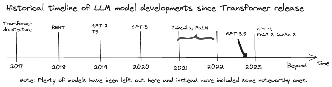
As we can see lots of interesting progress has been made in this space since the intial release of the Transformer paper. It’s worthwhile noting that the core compononents behind the transformer itself had been theorised around 15-20 years prior by the likes of Yoshua Bengio with subsequent work by others further developing on the ideas. The culmination of these ideas packaged in a novel implementation (self attention, transformer blocks etc) applied to the problem of translation (which performed well) was the key achievement.
In this section we’ll go into the specifics of trying to understand how these models work by diving into their internal mechanisms. A key point to remember is even though they all leverage the transformer architecture the use cases of each of the models is different.
The Transformer
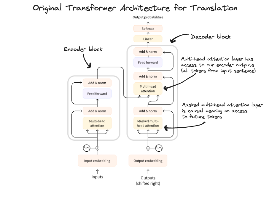
As you can see the transformer architecture itself involves many smaller parts all of which we will touch on in the coming sections.
Attention Mechanism
The first major step in our journey of understanding is mastering the attention mechanism which was one of the key breakthroughs presented inside the transformer paper. It’s helpful to use visualisations when trying to understand what is happening under the hood, below I have created a quick view I tend to use.
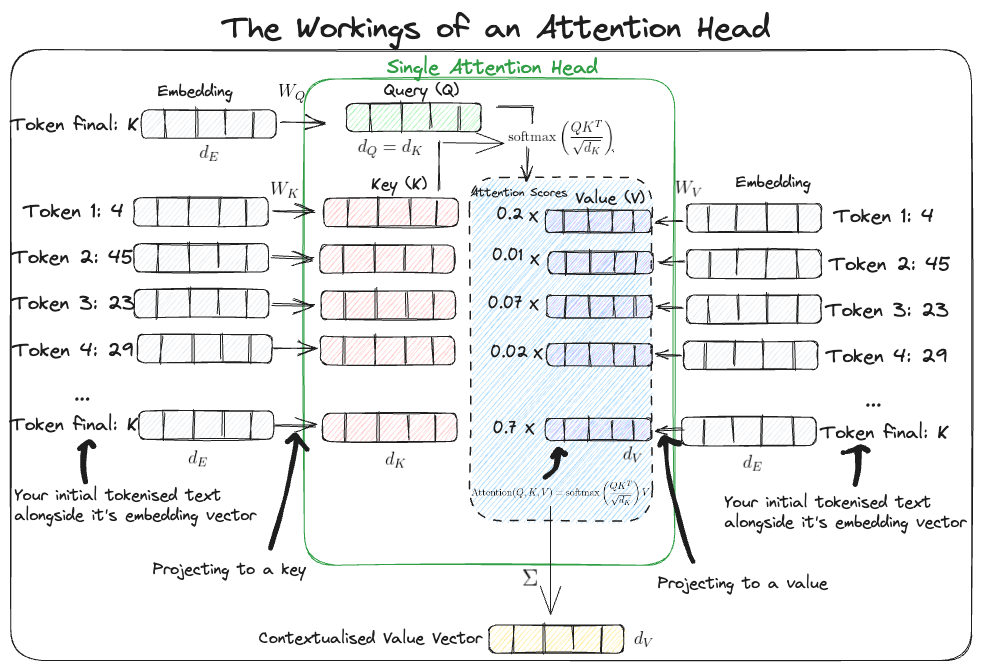
Essentially what this mechanism is doing is allowing the model to determine which positions in the input text (token positions) it should pay attention too in order to efficiently extract useful information all while ignoring irrelevant detail.
This is in stark contrast to RNN layers which try to build up a generic hidden state via the hidden vector which only captures an “overall representation” of the input at each timestep. Therefore as you unravel the layer and work your way through the various timesteps you’ll likely find that many words which aren’t relevant would have been picked up and encoded into the hidden vector in some way or another, something which attention heads don’t suffer from since it can decide (via the attention scores) which words are relevant and choose how to utilise that accordingly.
As we have seen above this is done utilising queries keys and values. As you may have guessed these concepts are analogous to retrieval systems (such as search engines) whereby you have a query and you want to “retrieve” the most relevant content i.e values based on how the query aligns with the keys (like a database index key).
In this context the query $Q$ can be thought of as a representation of your current task (e.g predicting the next token) which in this case is derived from the embedding of the final word in your input text by applying a weight matrix $W_Q$ to it. This weight matrix like others we’ll discuss acts as a map between the vector space of our embedding vectors and query vector. This is done in a way to ensure the query has the same dimensions as the keys $d_Q = d_K$ as we well see in a minute.
The key vectors $K$ are a representation of each of the words in the text. You can interpret these as descriptions of the kinds of prediction tasks each word can help you with. These can be derivived in a similar fashion to the query vector by using a weight $W_K$ to map the embeddings to vectors of dimensions $d_K$.
Now inside the attention head itself each of the key vectors can be compared to the query vector in a pairwise fashion to see if it “aligns” with the query. To do this we need a similarity measure between two vectors for which we can use the dot product which gives us $QK^T$ where $Q$ is our query row vector and $K^T$ is our key row vector transposed i.e a key column vector. As you can see this is why our query and key vector were made to have the same dimensions (so that the dot product could be computed).
The resulting output is scaled by $\sqrt{d_K}$ to keep the variance of the vector sum stable (approx close to one) and a softmax is subsequently applied to ensure all attention weights sum to one. Remember this would give a single attention score for each key meaning in the end you’ll end up with a vector of attention scores for each key.
Note: If you have high dimensional non-zero vectors the dot product can potentially grow very large. When you then apply a softmax function this can lead to values very close to $1$ for large inputs and close to $0$ for small inputs meaning that if you don’t scale the vectors you could end up with large variation in attention scores for an individual key across attention heads.
We can now bring in the value vector \(V\) which are also representations of the words in the sentence. You can think of these as the unweighted contribtuions of each word (since they are calculated straight from the embedding vectors). You can get these from the embedding vectors just as before by passing them through a weight matrix $W_V$ to change the dimensionality of the embeddings to $d_V$. The dimensionality of these value vectors don’t have to be the same as the query and keys (multiplication doesn’t rely on it).
Putting this all together you can multiply the attention scores (weighted importance) by the value vectors to get the Attention as shown below for a given $Q$, $K$ and $V$
\[\text{Attention}(Q, K, V) = \text{Softmax}\left(\frac{QK^{T}}{\sqrt{d_{K}}}\right) V\]As a result you end up with multiple attention vectors of dimension $d_V$ (as given by the above equation). To obtain the final output vector from the attention head attenion vectors are summed element wise across each dimension still yielding a vector of dimension $d_V$.
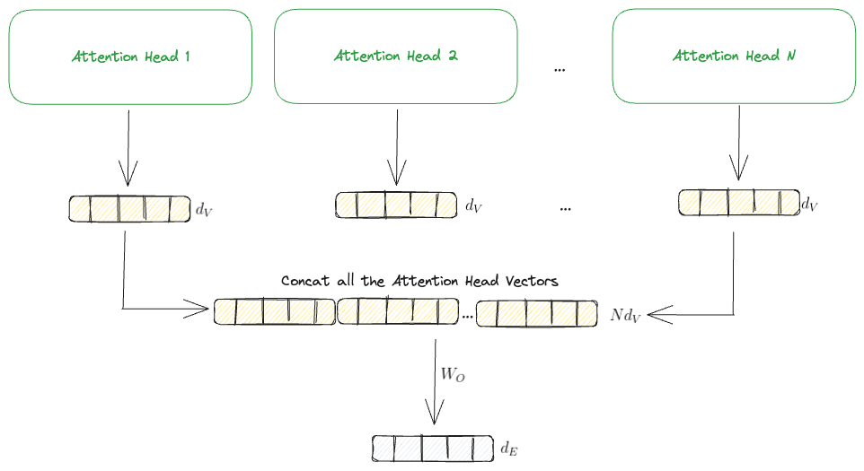
In reality though to improve performance an attention layer consists of multiple attention heads which are each independent of each other. Each one of these heads will follow the same process as outlined above to output a single attention head vector of dimension $d_V$. However, the subsequent layers of the transformers can’t work with these so instead we concatenate the vectors into a single vector and then multiply by another weight matrix $W_O$ to output a final vector of our desired size. I have provided a visual of this to make it alittle clearer.
Important: Now up until now we have thought of things at a token/word level where we have had a single query vector however in reality we have a whole text block which we want to predict the next token for. To do this we meed to consider each token position as a query vector simultaneously (this provides efficiency during training and is the way things are done in practice). This means instead of talking about the query, keys and values being vectors we instead need to represent them as matrices. All our intuitions still hold but you can imagine an extra dimension being included in the calculation depending on the number of tokens/words in our text. You’ll have to trust me that things pan out and the equations are exactly the same.
Here is what it would look like: $$ \begin{align} &\text{MultiHead($Q$, $K$, $V$)} = \text{Concat}(\text{head}^1, \dots,\text{head}^N) W_{O} \\ &\text{where head$^i$} = \text{Attention(QW$^i_Q$, KW$^i_K$, VW$^i_V$)} \\ \end{align} $$
Where the projections are parameter matrices: $$ \begin{align} &W^i_Q \in \mathbb{R}^{d_\text{model} \times d_Q} \\ &W^i_K \in \mathbb{R}^{d_\text{model} \times d_K} \\ &W^i_V \in \mathbb{R}^{d_\text{model} \times d_V} \\ &W^i_O \in \mathbb{R}^{Nd_V \times d_{\text{model}}} \\ \end{align} $$
and \(d_\text{model}\) is just our desired output size which is the same as our embedding size \(d_E\). This is then fed onto the next layer.
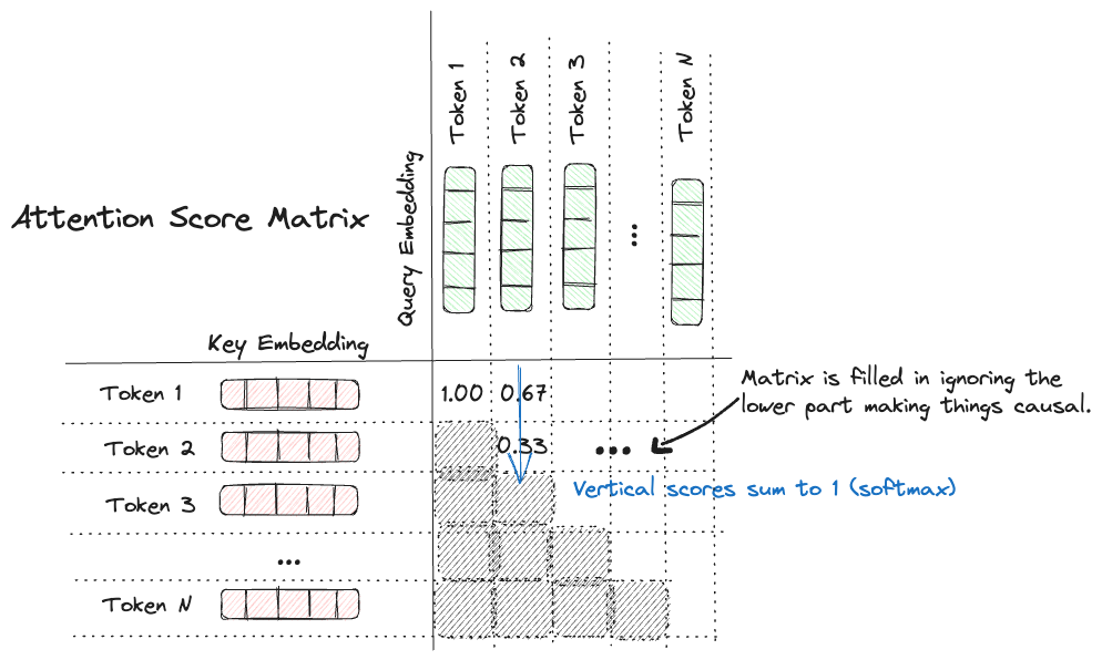
Causal Masking
Now for decoder based transformers it’s important no information leakage happens. To ensure this doesn’t happen a technique known as causal masking is employed. What this does is only consider tokens positionally prior to the given token as as potential key token. This masking can then be applied to the attention calculation. Mathematically this would be the same as computing a matrix of attention scores for all input query key combinations and only keeping the upper triangular part of the matrix (as shown below).
In code this would look something like the following:
def causal_attention_mask(batch_size, n_dest, n_src, dtype):
    """
    Performing the causal mask operation over tensors

    Parameters
    ----------
    batch_size: int
      The number of sequences in a batch
    n_dest: int
      Refers to the number of destination positions (or queries). These are the positions that will compute attention scores based on how relevant other positions (source positions) are to them.
    n_src: int
      Refers to the number of source positions (or keys). These positions are what the queries (destination positions) will attend to.
    dtype:
      The data type for the mask, typically tf.float32 or tf.int32

    Returns
    -------
    A lower triangualar tensor (matrix) where rows are queries and columns
    are keys. The dimensions of this tensor is flexible to batch size.

    Notes
    -----
    - n_dest usually equals n_src, have kept these separate to allow for playing around.
    """

    # Creating row and column indexes for our causal masks
    i = tf.range(n_dest)[:, None]
    j = tf.range(n_src)

    # Creating your mask where 1 represents the causally allowed
    # token positions and 0 represents those not allowed
    m = i >= j - n_src + n_dest
    causal_mask = tf.cast(m, dtype)
    causal_mask = tf.reshape(causal_mask, [1, n_dest, n_src])

    # Intermediate step to create multiplication array to tile
    # the mask array
    mult = tf.concat(
        [tf.expand_dims(batch_size, -1), tf.constant([1, 1], dtype=tf.int32)], 0
    )
    return tf.tile(causal_mask, mult)

# Viewing the causal masking for a single batch
np.transpose(causal_attention_mask(1, 10, 10, dtype=tf.int32)[0])
The above function is the reverse of what I described above in the sense that the query vectors are the rows of the matrix and the keys are the columns. This is why the np.transpose operation is performaned to make it upper triangular as described above.
Note: Attention Masks in general don’t need to be causal and only is so within the decoder attention mechanism to prevent chronological information leakage. In such cases it’s typically used to identify tokens such as start, stop & padding tokens which shouldn’t be attended too but are created to ensure valid tensor shapes when batching together multiple input sequences. More info can be found on the HuggingFace glossary page.
Embedding
In essence this is just the process of mapping your tokens to a sequence of vectors known as your embeddings. This mapping is a learnable process during training time or can be taken from an existing model (utilising the same pre-trained mapping). Here we make use of the Embedding layer provided by TensorFlow to demonstrate this.
I am glossing slightly over this since it isn’t the most exciting thing about transformers (although important) however I have added below some further reading which can provide more details:
- Great post providing intuition on Word Embeddings
- Showcases diagrams on how to interpret the process of creating the embeddings.
- Sentence-Transformer Repo
- Provides state of the art methods for creating embedding representations.
- HuggingFace blog post on embeddings
- Additional details on using embedding datasets.
Positional Encoding
Now there is a subtle point we have missed up until now. When the parallel operations are performed in the multi-head attention layer (each token acts as a query and gets dotted with the remaining text keys (in a causal manner as discussed above), this happens simultaneously) however in this lies a problem. We need the attention layer to be able to differentiate between the ordering of these operations especially if we are performing them in parallel.
To solve this a technique called positional encoding is performed when creating inputs to feed into the Transformer block. Instead of just performing the standard token embedding the position of each token (i.e it’s index if you imagine an array) is encoded using a position embedding.
In the same way a standard Embedding layer is used to convert the tokens into an a learned embedding vector the same layer can act on the positional index of each token. To then form the joint token-position embedding each of the respective embeddings are summed element wise meaning you end up with a final resultant vector which captures the positional information too.
Here is sample code for performing this:
class TokenAndPositionEmbedding(tf.keras.layers.Layer):
    def __init__(self, max_len, vocab_size, embed_dim):
        super(TokenAndPositionEmbedding, self).__init__()
        self.max_len = max_len
        self.vocab_size = vocab_size
        self.embed_dim = embed_dim
        self.token_emb = tf.keras.layers.Embedding(
            input_dim=vocab_size, output_dim=embed_dim
        )
        self.pos_emb = tf.keras.layers.Embedding(input_dim=max_len, output_dim=embed_dim)

    def call(self, x):
        maxlen = tf.shape(x)[-1]
        positions = tf.range(start=0, limit=maxlen, delta=1)
        positions = self.pos_emb(positions)
        x = self.token_emb(x)
        return x + positions

    def get_config(self):
        config = super().get_config()
        config.update(
            {
                "max_len": self.max_len,
                "vocab_size": self.vocab_size,
                "embed_dim": self.embed_dim,
            }
        )
        return config
As per the original transformer paper this would look slightly different where the transformation takes the following functional form:
\[\begin{align*} \text{P}(i,2j) &= \sin \left(\frac{i}{10000^\frac{2j}{d_{E}}}\right) \\ \text{P}(i,2j+1) &= \cos \left(\frac{i}{10000^\frac{2j}{d_{E}}}\right) \end{align*}\]Where these represent the elements \(\text{P}_{ij}\) of our positional encoding matrix \(\textbf{P}\). This matrix is then added in the standard fashion \(X + P\) to our given input \(X \in \mathbb{R}^{n \times d_{E}}\) which is our standard embedding matrix. Here \(n\) represents our sequence length.
The benefits of using these trigonometric functions in hindsight is multi-fold:
- To exploit their perodicity.
- In theory by being periodic you’ll get inherent encoding depending on the token positions which is what you’d want.
- Smoothness properties.
- Easier to learn for the model since the derivatives are well behaved.
- Precision of values.
- They have a nice range of values which allows you to have good control of the precision of the encoding process even as the context length grows.
A takeaway point is regardless of the form it’s important to encode positional information somehow as the model architecture itself doesn’t impose this by default. A nice response as to how this works can be found on the here.
Transformer Block
The Transformer itself is comprised of a Transformer Block component which consists of some skip connections, multi-head-attention layers, standard feed-forward layers and normalisations. Below is a nice visualisation of this.
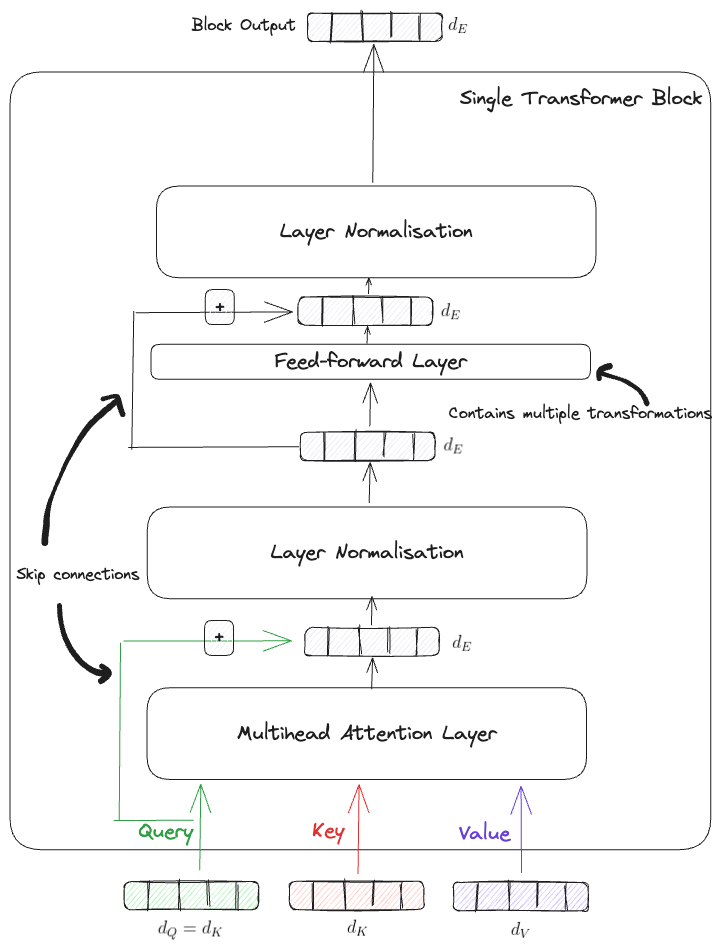
This block can be thought of as the fundamental unit from which the full transformer model is formed with which ultimatly just consists of copies of this block stacked ontop of each other.
It’s worth noting that no formal design constraints force the model to output matricies/vectors of the same dimension as intial embeddings however it is typically done to make this more consistent and simplify the design. This also helps ensure computational costs are more predictable as you start stacking blocks.
The purpose behind the skip connections, which are common in modern DNNs, is to allow for a “gradient free highway” to move information up the residual stream without interference and in turn also prevents things like the vanishing gradient problem.
By having dense feed-forward layers allows the model to extract nice higher level features and push those forward as the information goes deeper into the network.
The Layer Normalisation provides additional stabalisation to the training process (similar in a way to Batch Normalisation used in other architectures). However, they operate differently and are used in different contexts. Let’s dive into their differences, especially in the context of the Transformer architecture:
Batch Normalization (BatchNorm):
-
Operation: BatchNorm normalizes the activations across a batch for each feature independently. For a given feature, it computes the mean and variance across the batch and uses them to normalize the activations.
- Equation:
\(\begin{align}
&\mu_B = \frac{1}{m} \sum_{i=1}^{m} x_i
&\sigma_B^2 = \frac{1}{m} \sum_{i=1}^{m} (x_i - \mu_B)^2
&\hat{x}_i = \frac{x_i - \mu_B}{\sqrt{\sigma_B^2 + \epsilon}}
&y_i = \gamma \hat{x}_i + \beta
\end{align}\)
Where:
- $x_i$ is the input activation.
- $m$ is the batch size.
- $\mu_B$ and $\sigma_B^2$ are the mean and variance computed across the batch.
- $\hat{x}_i$ is the normalized activation.
- $\gamma$ and $\beta$ are learnable parameters.
- $\epsilon$ is a small constant to prevent division by zero.
- $y_i$ is the output of the batch normalisation.
-
Dimensions: BatchNorm requires a batch dimension. If you’re normalizing a
[batch_size, features]tensor, the mean and variance are computed across the batch dimension, resulting in a[features]sized tensor for both the mean and variance. - Usage: BatchNorm is commonly used in convolutional neural networks (CNNs). However, it’s less common in Transformer architectures because Transformers often deal with variable-length sequences, making consistent batch normalization challenging.
Layer Normalization (LayerNorm):
-
Operation: LayerNorm, on the other hand, normalizes the activations across features for each individual data point in the batch. In the context of the Transformer, it’s applied to the embeddings and the outputs of the self-attention mechanism.
- Equation:
\(\begin{align}
&\mu = \frac{1}{d} \sum_{i=1}^{d} x_i
&\sigma^2 = \frac{1}{d} \sum_{i=1}^{d} (x_i - \mu)^2
&\hat{x}_i = \frac{x_i - \mu}{\sqrt{\sigma^2 + \epsilon}}
&y_i = \gamma \hat{x}_i + \beta
\end{align}\)
Where:
- $x_i$ is the input activation.
- $d$ is the feature dimension.
- $\mu$ and $\sigma^2$ are the mean and variance computed across the features.
- The other symbols have the same meaning as in the BatchNorm equations.
-
Dimensions: LayerNorm does not require a batch dimension. If you’re normalizing a
[batch_size, features]tensor, the mean and variance are computed across the feature dimension, resulting in a[batch_size]sized tensor for both the mean and variance. - Usage: LayerNorm is extensively used in Transformer architectures. It’s applied before each sub-layer (self-attention or feed-forward neural network), and the output is passed through a residual connection.
Key Differences:
- Batch Dimension: BatchNorm operates across the batch dimension, while LayerNorm operates across the feature dimension.
- Dependency: BatchNorm’s behavior depends on the batch size and can be sensitive to it, while LayerNorm’s behavior is independent of batch size.
- Sequence Length: LayerNorm is more suitable for sequence data (like in Transformers) where the sequence length can vary across batches.
- Training Stability: LayerNorm tends to provide more stable training for Transformers compared to BatchNorm, especially when dealing with variable-length sequences.
In short, while both LayerNorm and BatchNorm aim to stabilize neural network training, they operate on different dimensions and are used in different contexts. LayerNorm is particularly well-suited for the Transformer architecture1.
The following article goes into further detail on this aswell as linking relevant resources.
Now, putting this all togther in code looks like:
class TransformerBlock(tf.keras.layers.Layer):
    def __init__(self, num_heads, key_dim, embed_dim, ff_dim, dropout_rate=0.1):
        super(TransformerBlock, self).__init__()
        self.num_heads = num_heads
        self.key_dim = key_dim
        self.embed_dim = embed_dim
        self.ff_dim = ff_dim
        self.dropout_rate = dropout_rate
        self.attention = tf.keras.layers.MultiHeadAttention(
            num_heads, key_dim, output_shape=embed_dim
        )
        self.dropout_1 = tf.keras.layers.Dropout(self.dropout_rate)
        self.ln_1 = tf.keras.layers.LayerNormalization(epsilon=1e-6)
        self.ffn_1 = tf.keras.layers.Dense(self.ff_dim, activation="relu")
        self.ffn_2 = tf.keras.layers.Dense(self.embed_dim)
        self.dropout_2 = tf.keras.layers.Dropout(self.dropout_rate)
        self.ln_2 = tf.keras.layers.LayerNormalization(epsilon=1e-6)

    def call(self, inputs):
        input_shape = tf.shape(inputs)
        batch_size = input_shape[0]
        seq_len = input_shape[1]
        causal_mask = causal_attention_mask(
            batch_size, seq_len, seq_len, tf.bool
        )
        attention_output, attention_scores = self.attention(
            inputs,
            inputs,
            attention_mask=causal_mask,
            return_attention_scores=True,
        )
        attention_output = self.dropout_1(attention_output)
        out1 = self.ln_1(inputs + attention_output)
        ffn_1 = self.ffn_1(out1)
        ffn_2 = self.ffn_2(ffn_1)
        ffn_output = self.dropout_2(ffn_2)
        return (self.ln_2(out1 + ffn_output), attention_scores)

    def get_config(self):
        config = super().get_config()
        config.update(
            {
                "key_dim": self.key_dim,
                "embed_dim": self.embed_dim,
                "num_heads": self.num_heads,
                "ff_dim": self.ff_dim,
                "dropout_rate": self.dropout_rate,
            }
        )
        return config
Feed-forward Layer
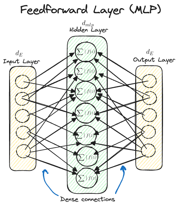
Again not super interesting but this can be thought of as just a standard MLP layer (typically a single hidden layer) which takes as input your prior tenors (associated with the prior layers output) performs a linear map to a higher dimensional space typically where \(d_{\text{mlp}} = 4 d_{\text{E}}\) where \(d_{\text{E}}\) is just the residual stream width \(d_{\text{model}}\) and then performs some non-linear activation and then maps back down to the residual stream size \(d_{\text{E}}\).
Intuitively this layer just continues feeding information foward and in doing so can impart useful additional features back to the residual stream (MLPs have shown to be great at this).
Un-embedding Layer
This is the final stage in the transformer model which maps the outputs from the transformer blocks to a tensor of logits representing the final output of your model. The nature of the logits ultimately depends on the specific type of model and use case you have and is sometimes callled the “language modelling head” of the model.
Encoder based models
The primary purpose behind encoder based models is to take in an input and build a representation of it (its features). This means that these models are optimized to acquire understanding from the input.
BERT
Here are some resources to assist in understanding how BERT works:
- Main BERT page on HuggingFace
- Comprehensive one stop shop page which provides various resources all centered around understanding and using BERT based models.
- Medium article explaining BERT
- Gives a nice summary of BERT and it’s various components.
- Released in 2018 close to when BERT came out.
- HuggingFace blog post on BERT
- Provides ways in which BERT works in particular making use of opensource implementations available via HuggingFace.
Decoder based models
The primary purpose behind decoder based models is to taken in representations (features) along with other inputs to generate a target sequence. This means that these models are optimized for generating outputs.
GPT
OpenAI introduced GPT in June 2018 in a paper titled “Improving Language Understanding by Generative Pre-Training”. What they do is essentially pre-train a generative (decoder only) transformer in an unsupervised manner. Evolutions of this process eventually become the infamous “ChatGPT” model that everyone is familar with.
Given the various building blocks defined prior we can piece together a simplified GPT based transformer architecture as follows:
import tensorflow as tf

MAX_SEQ_LEN = 100
VOCAB_SIZE = 50000
EMBEDDING_DIM = 256
N_HEADS = 6
KEY_DIM = 256
FEED_FORWARD_DIM = 256

inputs = tf.keras.layers.Input(shape=(None, ), dtype=tf.int32)
x = TokenAndPositionEmbedding(MAX_SEQ_LEN, EMBEDDING_DIM, FEED_FORWARD_DIM)(inputs)
x, attention_scores = TransformerBlock(num_heads=N_HEADS, key_dim=KEY_DIM, embed_dim=EMBEDDING_DIM, ff_dim=FEED_FORWARD_DIM)(x)
outputs = tf.keras.layers.Dense(VOCAB_SIZE, activation='softmax')(x)
gpt_model = tf.keras.models.Model(inputs=inputs, outputs=[outputs, attention_scores])
gpt_model.compile(optimizer="adam", loss=[tf.keras.losses.SparseCategoricalCrossentropy(), None])
gpt_model.summary()
Encoder-Decoder models
The original transformer that was introduced contained both the encoder and decoder parts. Having both parts are useful in tasks like summarization, question and answering, translation etc.
T5
Here are some good resources for working with the T5 model:
- Google blog post on T5
- The original T5 blog post created by Google in Feb 2020.
- Contains additional context on it’s development and purpose aswell as links to the paper, code and a colab notebook for you to use.
- HuggingFace T5 implementation model docs
- Comprehensive overview of what T5 is and all required information to begin playing around with it using the transformer library.
Applications of Large Language Models
Large Language Models (LLMs) have found applications across a multitude of industries. Here’s a breakdown of some of those areas aswell as use cases where LLMs can help:
- Media and Entertainment
- Script-writing Assistance: LLMs can help scriptwriters by generating dialogue, suggesting plot twists, or enhancing character descriptions.
- Game Development: In video games, LLMs can be used for dynamic dialogue generation, making non-player characters (NPCs) more responsive and natural in their interactions.
- Healthcare
- Medical Consultations: LLMs can assist doctors in answering patient queries, offering preliminary diagnostic suggestions based on patient symptoms, or directing patients to appropriate care resources.
- Medical Literature Review: LLMs can parse through vast databases of medical literature, summarizing findings, and assisting researchers in staying up-to-date.
- Legal Industry
- Contract Review: Automating the process of scanning contracts for discrepancies, missing clauses, or potential legal pitfalls.
- Legal Queries: Assisting clients with general legal information or directing them to the appropriate legal help.
- Education
- Tutoring Assistance: LLMs can assist students with questions about specific subjects, helping with homework or clarifying doubts.
- Language Learning: Assisting learners in understanding new languages, providing translations, and correcting language exercises.
- E-commerce
- Customer Support: Assisting customers with queries, tracking orders, or addressing concerns in real-time.
- Product Descriptions: Automatically generating or enhancing product descriptions based on specifications.
- Finance and Banking
- Financial Queries: Assisting clients with queries regarding their accounts, transactions, or general banking services.
- Financial News Summarization: Offering summaries or insights from long financial reports or news.
- Publishing
- Content Enhancement: Suggesting improvements, rephrasing, or generating content for writers.
- Fact-checking: LLMs can be trained to verify claims against a known database of facts, assisting journalists and writers.
- Real Estate
- Property Descriptions: Generating descriptive and engaging listings for properties based on key features and photos.
- Client Queries: Answering potential tenant or buyer questions about properties, amenities, or the surrounding area.
- Travel and Hospitality
- Travel Itinerary Planning: LLMs can suggest travel plans, attractions, or dining options based on user preferences.
- Hotel Customer Service: Answering guest queries about services, amenities, local attractions, and more.
- Research and Development
- Literature Review: Parsing through vast datasets of research literature and summarizing findings.
- Brainstorming: Offering ideas or potential directions for researchers based on existing knowledge.
- Manufacturing
- Technical Documentation: Assisting in generating or editing technical manuals and documents.
- Safety Protocols: LLMs can be trained to review safety procedures and recommend best practices.
The potential of LLMs is vast, and this list just scratches the surface. The versatility of these models allows them to be adapted and fine-tuned for specific needs across various industries and certainly more areas will come and go as time goes on.
Challenges and Limitations of Large Language Models
Here are some of the major ones alongside current solutions:
- Resource Consumption and Environmental Concerns:
- Training LLMs demands massive computational power, which translates to high energy use, leading to environmental concerns. Their carbon footprint is a point of contention in the AI community.
- Bias and Ethical Concerns:
- LLMs are trained on vast swathes of internet text, so they might inadvertently learn and perpetuate societal biases present in that data. They might produce discriminatory, biased, or politically insensitive content, which raises ethical concerns.
- Transfer of Learning and Generalization:
- While LLMs can handle a broad array of tasks, they might not always generalize well to specific tasks without fine-tuning or further training.
- Dependency on Large Amounts of Data:
- LLMs need huge datasets to train effectively, which might not always be available or feasible for every application.
- Interpretability:
- Understanding why LLMs make certain decisions or predictions remains a challenge. This black-box nature makes it hard to trust them in critical applications, such as healthcare or judiciary.
- Economic and Job Market Impact:
- The widespread use of LLMs might lead to job displacement in certain sectors, creating socio-economic challenges.
- Over-reliance and Trust:
- Over-relying on LLMs without understanding their limitations could lead to misinformation or faulty decision-making. For instance, taking medical or legal advice from an LLM without expert verification can be risky.
- Security and Misuse:
- There’s potential for misuse of LLMs, such as generating fake news, spamming, or crafting persuasive misinformation campaigns.
- Cost of Deployment:
- Although models like GPT-4 are powerful, deploying them for real-time applications might be costly in terms of computational resources.
- Lack of Creativity and Nuance:
- While LLMs can generate coherent text, they don’t truly understand context, culture, or human emotions. Thus, they may lack the creativity, nuance, or emotional intelligence inherent in human communication.
- Catastrophic Forgetting:
- When LLMs are fine-tuned on specific tasks, there’s a risk they might “forget” some of the vast knowledge they’ve been originally trained on, limiting their general applicability.
- Feedback Loops:
- If LLMs are used to generate content that’s later used to train newer versions of the model, it might create feedback loops where the model reinforces its own generated biases.
For LLMs to see broader acceptance and trust, addressing these challenges is critical. As the AI community is well-aware of these issues, ongoing research aims to alleviate many of these limitations.
Working with Large Language Models: A Practical Guide
In practice when you want to work with LLMs you won’t want to implement them from scratch.
Here is a short simple guide for working with LLMs to get you started:
- Understand Your Objective:
- Define your goals. Do you want to generate text, classify content, translate languages, or answer questions? Your goal determines the model type you’ll need.
- Basics of LLMs:
- Spend time understanding what LLMs are. They are pre-trained models on vast amounts of text data and can be fine-tuned to specific tasks.
- Choose the Right Model:
- Many pre-trained models are available. Depending on your objective, you might select from models like GPT (for text generation), BERT (for classification), or T5 (for multiple tasks).
- Setting Up Your Environment:
- Ensure you have Python installed.
- Install required libraries:
- You can make use of the Transformer library alongside PyTorch.
pip install transformers torch
- Use Open-Source Platforms:
- HuggingFace’s Transformers: This library provides easy-to-use APIs for many state-of-the-art LLMs. - Access the model hub: HuggingFace Model Hub - Explore and select the model that suits your needs.
- Load and Use a Model:
- Here’s a basic example using GPT-2 for text generation:
from transformers import GPT2LMHeadModel, GPT2Tokenizer tokenizer = GPT2Tokenizer.from_pretrained("gpt2-medium") model = GPT2LMHeadModel.from_pretrained("gpt2-medium") input_text = "Once upon a time" input_ids = tokenizer.encode(input_text, return_tensors="pt") output = model.generate(input_ids, max_length=100) generated_text = tokenizer.decode(output[0], skip_special_tokens=True) print(generated_text) - Fine-tuning:
- If you have a specific task, you might want to fine-tune a pre-trained model on your dataset.
- You’ll need annotated data for your task.
- Follow fine-tuning guides specific to your chosen model and task. HuggingFace provides training utilities to make this easier.
- Deployment:
- Once you’ve fine-tuned (if necessary), deploy your model using platforms like Flask for web APIs or integrate directly into your software.
- Consider efficient deployment using model quantization or onnx exports for optimized performance.
- Be Responsible:
- Remember LLMs can have biases or make incorrect predictions.
- Always verify the outputs and ensure they meet your application’s ethical and quality standards.
- Continuous Learning:
- The field of LLMs is rapidly evolving. Stay updated with new research, models, and best practices. HuggingFace’s community and forums are excellent resources.
Perhaps further details on this will be the topic of future posts 🙂
Conclusion: Reflection
So hopefully this whirlwind tour of LLMs has been insightful. We have:
- Defined LLMs and observed the current SOTA architectures which are powering these models.
- Performed a deep dive on some of the maths behind aspects of these models and implemented some code for them.
- Descibed some use cases of LLMs across indsutries and touched on some of the major challenges faced with them too.
- Touched on ways to play with variants of these models to solve your particular problems (utilising HuggingFace).
Reference Material & Further Reading
- Practical (Implementation)
- Creating custom TensorFlow components
- Alot of the code here requires developing custom functions so it’s useful to understand the keras way of doing so via the subclassing API.
- Practicle NLP course by HuggingFace
- Great way to gain a practical experience working with the libary.
- Help solidify you understanding of Transformers and using for various tasks.
- Creating custom TensorFlow components
- Non-Practical (Intuition)
- Mathematical Framework for Transformer Circuits
- Fairly comprehensive overview of the mathematical underpinnings of simplified transformer components.
- Nice visuals which help in understanding how things flow through the model.
- Detailed Overview of LLMs (extended post)
- Nice since it touches on various aspects of LLMs along with resource links to learn more as you go along.
- TowardsDS Transformer Explantion post
- Good breakdown of how things work.
- Illustrated Transformer post
- Nice visuals which help in understanding how things flow through the model.
- Mathematical Framework for Transformer Circuits
-
The original GPT paper uses LayerNorm to prevent depenencies across batches however work by Shen et al shows that tweaking Batch Normalisation might not be too bad. ↩