Table of Contents
- Review
- Introduction
- Background
- Technical Details
- Key Highlights
- Applications
- Future Directions
- Conclusion
- Resources
Review
Before diving into the details of how KANs work it’s best to have some basic refreshers on key technologies which are required to have a better understanding.
We’ll touch on the following:
- MLPs
- Curve Fitting
- Bezier Curves
- Spline Functions
- B Splines
- Function Approximation
- Universal Approximation Theorem
MLPs
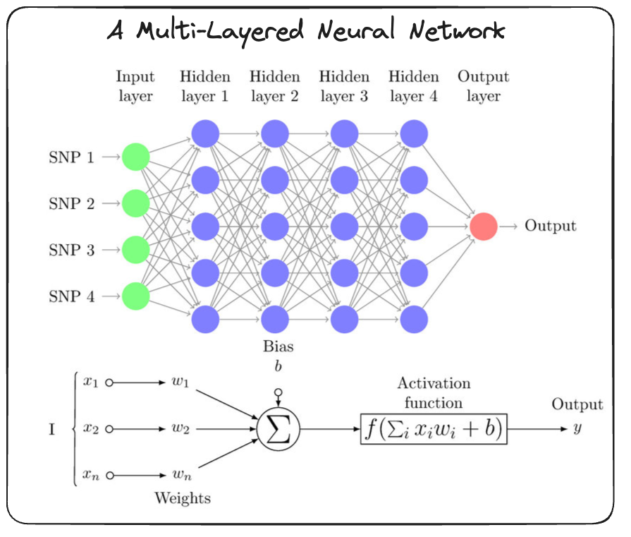
- Consists of multi layers filled with neurons.
- Typically all neurons are connected to all other neurons in whats known as a fully-connected manner.
- Mathematically each layer performs the following operations $y = xW^T + b$ which can be found on the PyTorch docs followed by some activation function $\sigma$.
- Where:
- $ W $ is the weight matrix of shape $(\text{out_features}, \text{in_features})$,
- $ b $ is the bias vector of shape $(\text{out_features})$, if
bias=True. - The output tensor $ y $ will have the shape $(N, *, \text{out_features})$.
- Where:
- The activation function is necessary in order to add in non-linearities, without it you wouldn’t be able to model complex things (as we’ll touch on later).
- As a thought experiment you can consider $ y_{1} = xW_{1}^T + b_{1}$ as being the output from a layer, if this is fed into another layer the linear composition becomes $ y_{2} = xW_{1}^TW_{2}^T + b_{1}W_{2}^T + b_{2}$ where you can see the behviour looks analogous to a single layers computation.
# Step 1: Create some dummy data
dummy_data = torch.randn(5, 3)
print("Dummy Data:\n", dummy_data)

# Step 2: Define a single linear layer
# Let's create a linear layer that maps from 3 features to 2 features
linear_layer = nn.Linear(in_features=3, out_features=2)

# Step 3: Apply the linear layer to the dummy data
output_data = linear_layer(dummy_data)
print("\nOutput Data:\n", output_data)
Curve Fitting
The objective here is given a series of data points you want to be able to fit a curve through those points. In practice plenty of ways exist and we’re going to touch on some of these.
- Polynomial curve fitting.
- Given a set of $N$ points it’s possible to show that you can find a polynomial of degree $N-1$ which goes through these points, can check out here.
- You can solve for the coefficients of the polynomial by solving the system of linear simultaneous equations.
- This works well when you have a low number of points but can have some draw backs as the number of points increases.
- Computation: Can argue if you have millions/billions of recrods then solving for the coefficients of a high order polynomial is not efficient.
- Weird Behaviour: You might observe properties where by the polynomial isn’t tight about the points but almost forecfully made to go through the points, e.g might pass through a point but then shoot up rapidly before going through the next point. Ideally you’d like a relatively smooth transition.
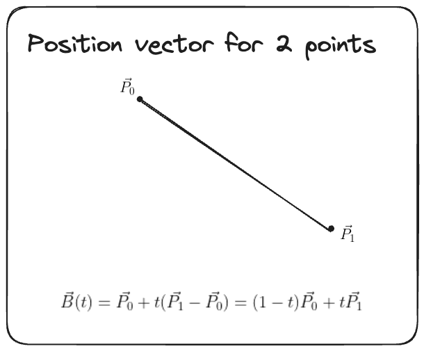
- Bezier Curves.
- Instead given any two points you can form a curve going through them by interpolating the distance by considering their position vectors $\mathbf{B}(t) = \mathbf{P_{0}} + t (\mathbf{P_{1}} - \mathbf{P_{0}}) = (1 - t) \mathbf{P_0} + t \mathbf{P_1}$.
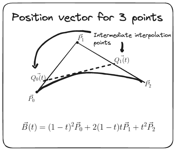
- Given three points this can be extended in a similar manner by interpolating the pairwise interpolation between points (1 and 2) and (2 and 3), can leave it for the reader to confirm that you get $\mathbf{B}(t) = (1-t)^2 \mathbf{P}_0 + 2(1-t)t \mathbf{P}_1 + t^2 \mathbf{P}_2$ for $\quad 0 \leq t \leq 1$.
- This can be generalised to an $n^{th}$ order Bezier curve for $n+1$ control points in the form $\mathbf{B}(t) = \sum_{i=0}^{n} \binom{n}{i} (1-t)^{n-i} t^i \mathbf{P}_i$.
- Where:
- $0 \leq t \leq 1$ is the parameterised dummy variable.
- $\binom{n}{i} = \frac{n!}{i!(n-i)!}$ is the binomial coefficient.
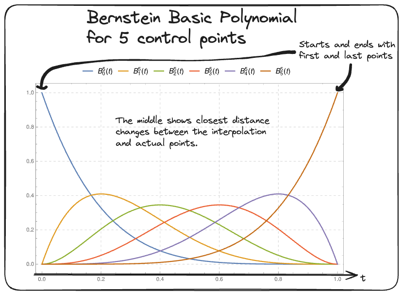
- $B_{i,n}(t) = \binom{n}{i} (1-t)^{n-i} t^i$ are the Bernstein Polynomials.
- Where:
- Best to think of the general form as being a “weighted sum of the control points”. where each Bernstein polynomial acts as the weighting for the control points helping inform us of the contribution of a given point to the final interpolated curve at some $t$.
- Again this is good and can provide a nice approximation but it can be quite expensive to compute if you have lots of data!
- Spline Functions
- Consists of piecewise polynomials over some given interval who’s degree corresponds to the highest degree of the polynomial parts, wiki has a description.
- You can split the interval into $k$ parts ($k+1$ points) which defines some Polynomial $P_i$ to each of these $k$ intervals. The set of $k+1$ points can be used to form a knot vector $\mathbf{t} = (t_{0}, …, t_{k})$ defining the boundary over which the interval splits are defined.
- A smoothness vector $r = (r_1,…,r_{k-1})$ exists which defines the smoothness (continuity) for each $t_i$ where $i = 1, …, k-1$ (number of points $k+2$ minus the $2$ for the edges)
- B-Splines
- Intuitively this utilises the notion of Bezier curves and Spline functions and applies low order Bezier Curves in a piecewise fashion and stiches togther the result, more here.
- Mathematically this looks something like $\mathbf{r}(t) = \sum_{i=0}^{n} N_{i,p}(t) \mathbf{P}_i$
- Where $N_{i,p}(t)$ are the B-spline basis functions and $P_i$ are the control points.
- The B-Spline basis functions can be calculated recursively and unlike the Bezier curves the degree of the curves isn’t completly dependent on the number of control points (which allows you freedom to decide).
- You can fix the degree of your B-Spline (same as the Bezier curve degree) to $k$ (order $k+1$) and then providing you have $n$ control points this gives you $n-k$ Bezier Curves to stich togther.
- E.g Say you have $4$ points and want to fit a $2^{nd}$ degree (Quadratic) Bezier curve then you’ll have $4-2=8$ Bezier curves.
- The points where the stiched polynomials (Bezier Curves) meet are called knots and are defined by the knot vector which specifies the values of t for which the curves join.
- Mathematically $\mathbf{T} = (t_0, t_1, t_2,..,t_{n+k})$.
- The knot analogy comes from the fact that it’s like joining bits of string togther.
- B-Splines have some nice properties:
- Flexibility and Smoothness: Higher-order B-splines (with higher k) can represent more complex shapes and provide smoother transitions between segments. However, they also require more control points.
- Since a $k^{th}$ order B-Spline with at most $C^{k-2}$ continutity at breakpoints meaning that as $k$ grows so does the strength of the continuity hence smoothness properties.
- Local Control: B-splines provide local control over the curve shape, meaning that moving a control point affects only a portion of the curve, unlike Bézier curves which have global control.
- This comes from the fact that B-Spline curve consists of segments meaning if you move a partiuclar control point $\mathbf{P}_i$ only a portion the curve interpolated around there would be impacted.
- Flexibility and Smoothness: Higher-order B-splines (with higher k) can represent more complex shapes and provide smoother transitions between segments. However, they also require more control points.
Universal Approximation Theorem
At their core neural networks are function approximators. In the case of ML given some data we often like to make certain predictions and when doing so the assumption is there exists some unknown true function which maps from the input features to the target and by training your neural network you are trying to best approximate that true unknown function.
At this point you might be wondering “Why is this even worthwhile?” and “What gives us the reason to believe the neural net will make any progress?”. The key to answer this lies in the universal-approximation theorem which theoretically shows “Given a neural network of a certain depth (number of layers) and width (number of neurons) it can be used to approximate any continuous function if using specific non-linear activation functions.”.
In other words if you have some data (consisting of features and a target) and a true relationship exists between them then a sufficiently large neural network would be able to get sufficiently close to that unknown function within a given error rate $\epsilon$.
This shows that there is merit in trying to use neural networks to perform modelling in ML.
Now before everyone starts trying to use neural nets to predict the future there are some caveats.
- These are theoretical bounds and provides no strict guidance on architectural requirements.
- The exact choices of parameters is fine grained and changes problem to problem.
- Practically things might turn out to be costly.
- For a given dataset it’s hard to know how much the hardware would cost to provide sufficient approximations for any given problem.
- GPUs are not cheap.
- Computer limitations
- Your hardware might not be able to hold the weights to the required precision.
- Data
- You assume that a true relationship exists, sometimes it might not.
Introduction
- Overview: Briefly introduce Kolmogorov-Arnold Networks (KANs) and their significance in the field of machine learning.
- Objective: State the purpose of the investigation, which is to understand the theoretical foundations, practical applications, and potential benefits of KANs.
Kolmogorov-Arnold Networks (KANs) represent a novel approach to neural network design, inspired by the Kolmogorov-Arnold representation theorem. This investigation aims to explore the theoretical foundations, practical applications, and potential benefits of KANs, providing a comprehensive understanding of their capabilities and limitations.
The recent paper is one of the key reasons for the resurection of this space as they mention:
“Our contribution lies in generalizing the Kolmogorov network to arbitrary widths and depths, revitalizing and contexualizing them in today’s deep learning stream, as well as highlighting its potential role as a foundation model for AI + Science.” - Ziming Liu, KAN paper leading author
A quick timeline shows:
- 1957
- Invention of the perceptron, Frank Rosenblatt.
- Kolmogorov-Arnold Representation, A.N. Kolmogorov.
- 1975
- Original Kolmogorov networks coined by Robert Hecht-Nielsen, paper link
- 2024
- Kolmogorov-Arnold Networks (resurface), Ziming Liu et al.
Background
- Kolmogorov-Arnold Representation Theorem:
- Explain the theorem and its historical context.
- Discuss how the theorem provides the foundation for KANs by allowing the decomposition of multivariate functions into univariate functions.
- Comparison with Multi-Layer Perceptrons (MLPs):
- Highlight the differences between KANs and traditional MLPs, focusing on activation functions and network architecture.
The Kolmogorov-Arnold representation theorem, formulated by Andrey Kolmogorov and Vladimir Arnold, states that any multivariate continuous function can be represented as a finite composition of univariate functions.
The general form of the Kolmogorov-Arnold representation for a function $f: [0, 1]^n \to \mathbb{R}$ can be written as: \(f(x_1, x_2, \ldots, x_n) = \sum_{q=1}^{2n+1} \Phi_q \left( \sum_{p=1}^{n} \phi_{q,p}(x_p) \right)\)
where:
- $ \Phi_q: \mathbb{R} \to \mathbb{R} $ are continuous functions,
- $ \phi_{q,p}: [0,1] \to \mathbb{R} $ are continuous functions,
- $ x_1, x_2, \ldots, x_n $ are the input variables.
In laymans terms it shows that “the only true multivariate function is addition since all other functions can be written using the sum of univariate functions”.
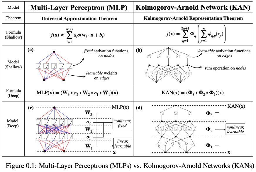
This theorem provides the basis for KANs, which decompose complex functions into simpler, learnable components. Unlike traditional MLPs, which use fixed activation functions on nodes, KANs employ learnable activation functions on edges, offering greater flexibility and efficiency.
Here is a nice table to summarise the difference between both KANs and MLPs, the key things to point out are:
- Different theorem used for underlying the architecture.
- Instead of multiplying input features by weights you instead run these through a function.
Technical Details
- KAN Architecture:
- Describe the structure of KANs, including the use of spline-parametrized univariate functions instead of traditional linear weights.
- Explain how KANs replace fixed activation functions with learnable activation functions on edges.
- Theoretical Guarantees:
- Summarize the theoretical advantages of KANs, such as faster neural scaling laws and the ability to represent complex functions with fewer parameters.
- Implementation:
- Discuss the implementation details.
- Mention any specific libraries or tools used in the implementation.
KAN Architecture
Here we can take a look at a standard KAN network with 2 input features to get an understanding of the KART theorem.
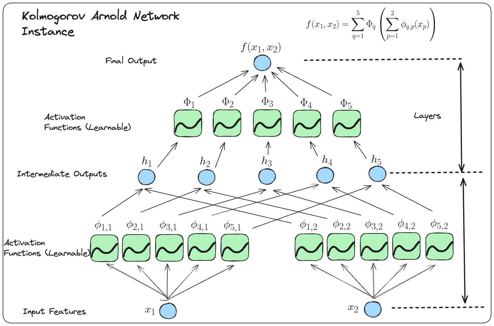
To spot how to generalise to form KAN networks it’s worthwhile to write the Kolmogorov-Arnold representation in matrix form:
\[f(x)={\bf \Phi}_{\rm out}\circ{\bf \Phi}_{\rm in}\circ {\bf x}\]where
\[{\bf \Phi}_{\rm in}= \begin{pmatrix} \phi_{1,1}(\cdot) & \cdots & \phi_{1,n}(\cdot) \\ \vdots & & \vdots \\ \phi_{2n+1,1}(\cdot) & \cdots & \phi_{2n+1,n}(\cdot) \end{pmatrix},\quad {\bf \Phi}_{\rm out}=\begin{pmatrix} \Phi_1(\cdot) & \cdots & \Phi_{2n+1}(\cdot)\end{pmatrix}\]As you can see the $\Phi_{in}$ represents the inner functions and the $\Phi_{out}$ represents the outer functions. Since we define a layer as taking in some input features and giving out some output features we can say “the Kolmogorov-Arnold representations are simply compositions of two KAN layers”.
Going further with this we notice that both \({\bf \Phi}_{\rm in}\) and \({\bf \Phi}_{\rm out}\) are special cases of the following function matrix \({\bf \Phi}\) (with \(n_{\rm in}\) inputs, and \(n_{\rm out}\) outputs), we call this general form a Kolmogorov-Arnold layer with dimensions \(n_{out} \times n_{in}\):
\[{\bf \Phi}= \begin{pmatrix} \phi_{1,1}(\cdot) & \cdots & \phi_{1,n_{\rm in}}(\cdot) \\ \vdots & & \vdots \\ \phi_{n_{\rm out},1}(\cdot) & \cdots & \phi_{n_{\rm out},n_{\rm in}}(\cdot) \end{pmatrix}\]\({\bf \Phi}_{\rm in}\) corresponds to \(n_{\rm in}=n, n_{\rm out}=2n+1\), and \({\bf \Phi}_{\rm out}\) corresponds to \(n_{\rm in}=2n+1, n_{\rm out}=1\).
After defining the layer, we can construct a Kolmogorov-Arnold network simply by stacking layers! Let’s say we have $L$ layers, with the \(l^{\rm th}\) layer ${\bf \Phi}_l$ have shape \((n_{l+1}, n_{l})\). Then the whole network is
\[{\rm KAN}({\bf x})={\bf \Phi}_{L-1}\circ\cdots \circ{\bf \Phi}_1\circ{\bf \Phi}_0\circ {\bf x}\]In constrast, a Multi-Layer Perceptron is interleaved by linear layers ${\bf W}_l$ and nonlinearities $\sigma$:
\[{\rm MLP}({\bf x})={\bf W}_{L-1}\circ\sigma\circ\cdots\circ {\bf W}_1\circ\sigma\circ {\bf W}_0\circ {\bf x}\]Note: I find it’s nice to refer to pages 4 and 5 of the acutal paper as it provides a more detailed explaination of the notation alongside some nice plots.
KANs are designed with a unique architecture that replaces traditional linear weights with spline-parametrized univariate functions (details referenced below).
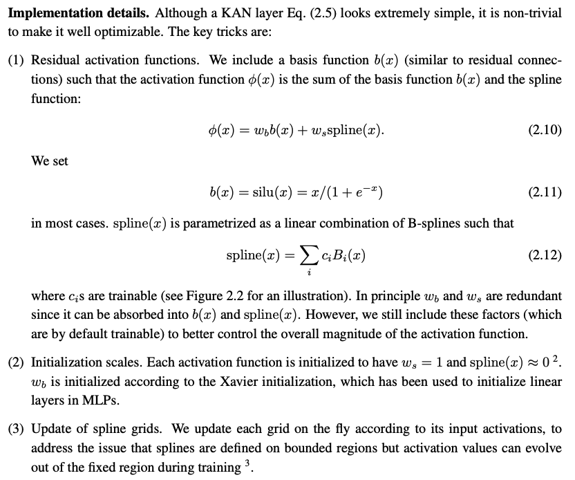
Key takeaways are:
- The activation function is learning only from the spline part (the other part is static).
- Once you set the number of control points and degree of the underlying Bezier curves the B-Spline weightings become fixed meaning you only care about learning where to put the control points.
- As the network learns different activation functions might end up learning and settling on different positions for the control points based on the input features.
This allows KANs to dynamically learn activation patterns, leading to improved accuracy and interpretability. The theoretical guarantees of KANs include faster neural scaling laws and the ability to represent complex functions with fewer parameters.
Theoretical Guarantees
Here is a view of the parameter efficiency between the two.
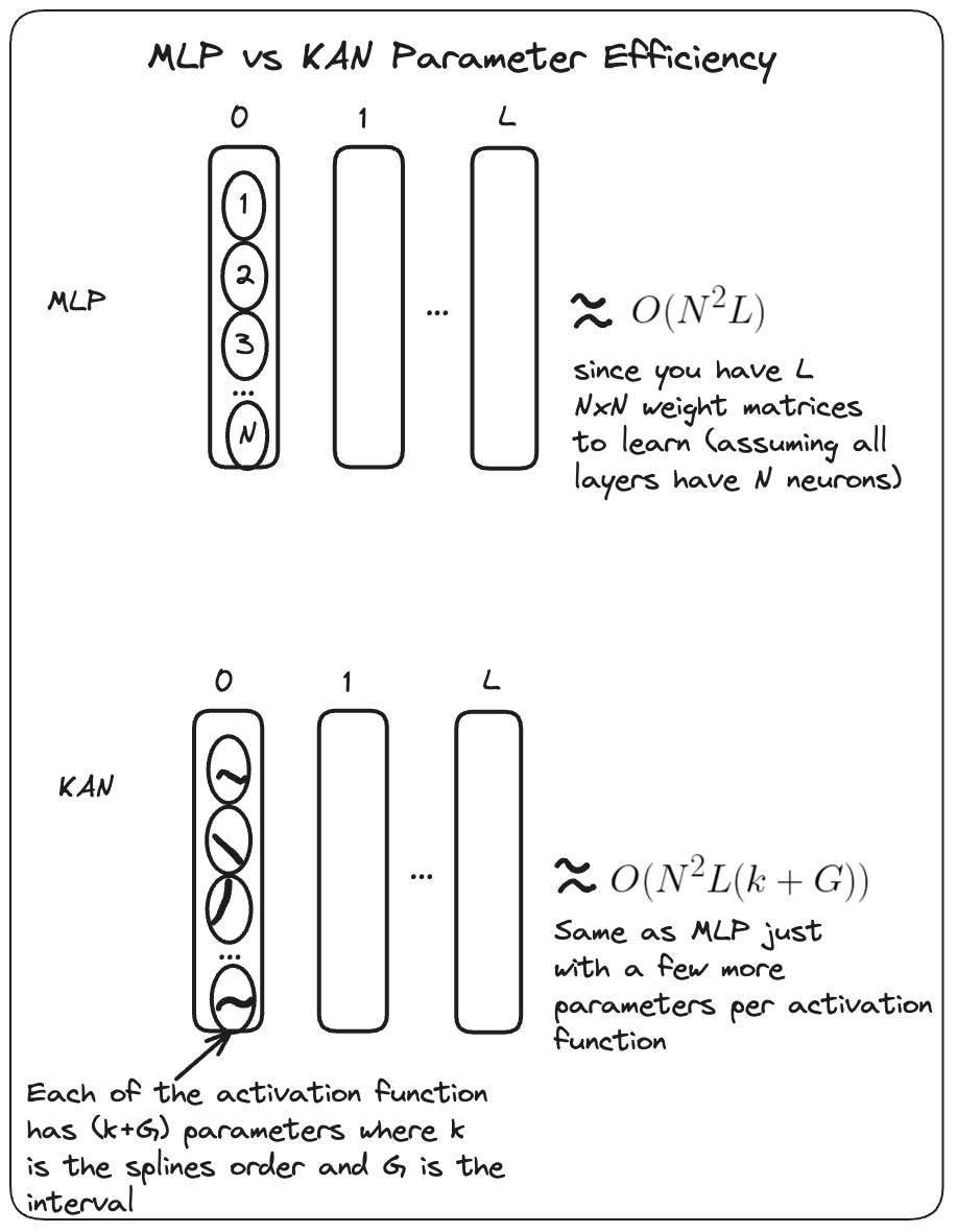
As you can see KANs do have more parameters however in practice you need a much smaller $N$ than MLPs to maintain/ exceed the accuracy on certain tasks. - This results in a parameter saving gain while still maintaining generalisation capabilities. - They statement was made after they showed they beat deepminds $3 \times 10^{5}$ parameter MLP on a task in Knot theory with a $2 \times 10^{2}$ parameter KAN while still maintaining a higher $81.6$% accuracy vs $78$% for the MLP.
Implementation
We can make use of the pykan library to peform some tasks with KAN networks.
They provide both an implementation of the algorithm along with helper functions for common tasks. We can take a look at the process of approximating a simple symbolic equation.
- Create dataset consisting of inputs and outputs.
- Instantiate the model and apply it to your dataset.
- Plot the learnt model graph.
- Prune the network to remove non significant activations.
- Plot the new pruned graph.
- Automatically view the most appropriate setting functions on top pruned activations.
- Obtain the resulting symbolic expression.
# Create dataset
f = lambda x: torch.exp(torch.sin(torch.pi*x[:,[0]]) + x[:,[1]]**2)
dataset = kan.create_dataset(f, n_var=2)
dataset['train_input'].shape, dataset['train_label'].shape

# train the model
# create a KAN: 2D inputs, 1D output, and 5 hidden neurons. cubic spline (k=3), 5 grid intervals (grid=5).
model = kan.KAN(width=[2,5,1], grid=5, k=3, seed=0)
model.train(dataset, opt="LBFGS", steps=20, lamb=0.1);
model.plot()
model = model.prune()
model(dataset['train_input'])
model.plot()

# Fix values
model.auto_symbolic()

# obtaining symbolic formula
formula, variables = model.symbolic_formula()
formula[0]
Key Highlights
- Experiments:
- Summarize the results of numerical experiments showing the accuracy, interpretability & efficiency improvements of KANs over MLPs.
- Challenges:
- Discuss the potential challenges and limitations, such as the complexity of training and the need for smoothness in univariate functions.
KANs offer several advantages, including improved accuracy, interpretability, and efficiency over a number of varying examples. However, they also present challenges, such as the complexity of training and the need for smoothness in univariate functions. Addressing these challenges is crucial for the successful implementation of KANs.
Interpretability
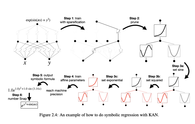
An intesting application is to Symbolic regression where the aim is to approximate a known closed form function using a KAN.
The highlevel steps are:
- Train with regularization to introduce sparsity to activation functions.
- Prune those functions.
- Fix the activation functions based on there appearance up until that point.
- Re-train affine parameters defined as part of function fixing.
- Ouput symbolic formula.
This shows the network was intrinsically able to learn the function inside some of these learnable activations using just the training data. This is alot more interpretable than normal MLPs as we as humans are able to verify things much easier when observing functions rather than just arrays of numbers.
- The reason for KANs being good at Symbolic regression is still a boundary to be explored but it can be argued it’s all down to inductive biases.
- This can be understood interms of a thought experiment. If a task is generated by a KAN network then a student KAN network would perform better than another network (say MLP).
- This in turn suggests the reason for good KAN performance on things like symbolic formulas is that KANs inductive bias aligns with that of the tasks.
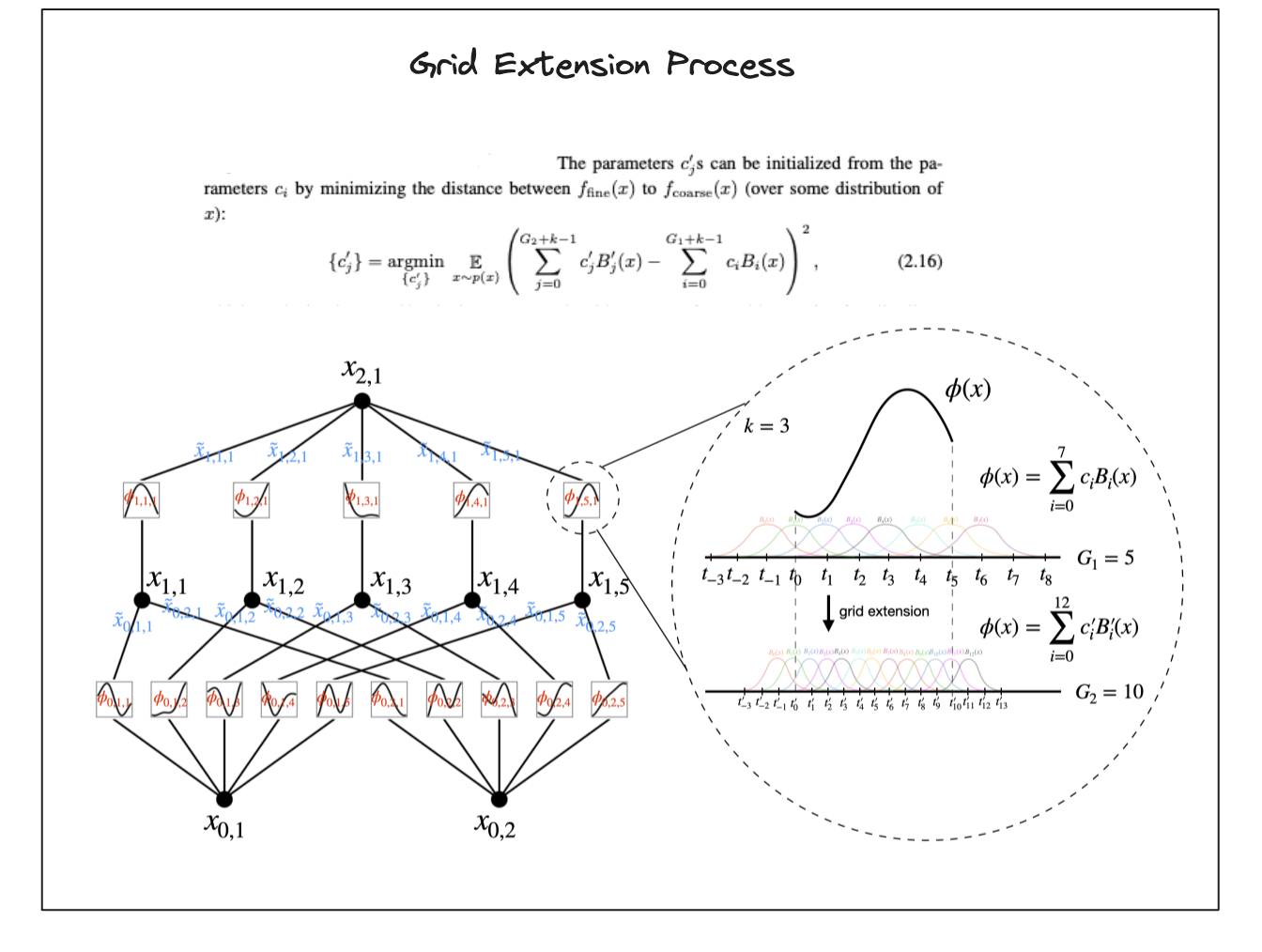
Accuracy (Grid Extension)
- If you want to get better approximations for your KANs you can increase the number of control points (grid points).
- By doing so your making your activation functions gain more expressive power by increasing the accuracy of the spline calculation.
- You can imagine this as increasing all of your control points from say $3$ to $7$ which can allow you to learn the $\sin$ function.
- $3$ points wouldn’t allow you to model the $\sin$ function.
- This is nice since you don’t need to change the structure of the network to improve the expressiveness.
- For MLPs you’d have to widen your network (hence increasing the number of parameters) which can make things less efficient.
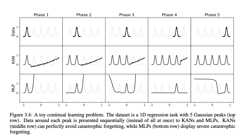
Accuracy (Continual Learning)
- The below experiment showcases how MLPs forget and perform poorly on old tasks as they are trained on new ones.
- The suspected reason for this is the global activation functions can propagate local changes far through the network.
- The KAN network can overcome this thanks to the spline locality properties.
- The behaviour around a specific region is controlled by the control points near that region, control points far away from that region don’t impact as much.
- As you feed in more data only the control points near the data values that you feed in are changed.
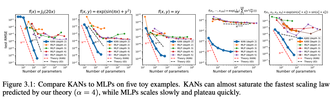
Efficiency (Scaling)
- KANs show promise on scaling when tested on toy function appromixations (inline with theoretical results).
- General scaling laws take the form $l \propto N^{- \alpha}$ where $l$ is the approxmate error, $N$ is the number of parameters and $\alpha$ is the scaling exponent.
- For approximating a d-dimensional function in general a uniform order $k$ spline would have a scaling law $l \propto N^{- \frac{(k + 1)}{d}}$.
- Assuming a smooth KAN representation the equivalent scaling law for a KAN would be $l \propto N^{- (k + 1)}$ since $d=1$ from KART.
- This is important as certain context favour models with promising scaling laws.
- Such as in the LLM space good scaling laws means throwing more compute can continue to improve performance.
Applications
- When to use:
- Explain in what scenarios KANs can be used for.
- What areas to use
- Touch on some potential areas that might be useful to explore for the business.
Here is a quick guide on when to use each architecture depending on what you want to optimise on.
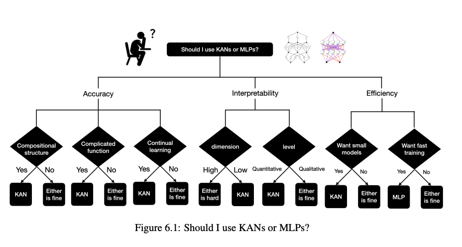
In general KANs seems like a worthwhile architecture to experiment with if you’re trying to find compositional structure that is interpretable within your data.
Some speculative applications for our business
- Interpretable Deep Learning Based Supervised Modelling
- Training a small model on a dataset to learn relations between features and outputs.
- Assuming some true relationship exists between your feature and targets this can help assess how they relate.
- MLP Replacement in RL Modelling
- Some policies are represented by neural networks.
- Replacing some of the layers with these MLP layers with KANs might improve accuracy along with parameter count efficiency.
Future Directions
- Research Opportunities:
- Identify areas for future research, such as further optimization of KAN architectures and exploration of new applications.
- Practical Implementations:
- Suggest practical steps for integrating KANs into existing machine learning workflows and systems.
- Advanced Architectures:
- Future research opportunities include further optimization of KAN architectures and exploration of new architectures thay build on this.
- This could incldude different types of arcitivation functions, making calculations more efficient.
- Creating hybrids with other architectures which address various shortcomes.
- Explainable AI
- Enhancing the interpretability of neural nets is highly important if trying to use in practice
- Development of tooling to visualise the structures would really help and lends itself to AI.
- Science + AI
- The authors showed KANs can be helpful assistants/collaborators for scientists by using them as a tool to help extract insights about physical problems.
Conclusion
- Summary:
- Recap the key points discussed in the investigation.
- Final Thoughts:
- Provide your insights on the potential impact of KANs on the field of machine learning and their relevance to EE.
In summary, KANs represent a promising alternative to traditional MLPs, offering improvements in accuracy, interpretability, and efficiency in specific problem domains. There potential impact on the field of machine learning is substantial not purely because of there improvement but because they provide a branch upon which alternative architectures can be explored.
Having said that from an industry perspective due to various technical subtlties it might be worthwhile waiting until more insights can be gathered and instead playaround in a more experimental way before trying to spend time productionising models with KANs.
“KANs are great”, but more of “try thinking of current architectures critically and seeking fundamentally different alternatives that can do fun and/or useful stuff. KANs and MLPs cannot replace each other (as far as I can tell); they each have advantages in some settings and limitations in others. I would be intrigued by a theoretical framework that encompasses both and could even suggest new alternatives” - Ziming Liu, KAN paper leading author
Resources
- Papers:
- Videos: