Table of Contents
- Introduction
- Detecting Differences in Distributions
Introduction
In data analysis, comparing columns of data across various splits can be likened to ensuring different sections of a pie have the same flavor and texture. Just as a chef wants each slice of a pie to taste the same, analysts aim for consistent feature distributions across dataset splits. This consistency is crucial for reliable inferences and predictions. In machine learning, datasets are commonly split into training, validation, and test sets. This practice assumes that feature distributions across these splits are similar. As a result understanding these distributions (along with strategies to discern differences) are highly useful. This blog post will share strategies to determine if a feature’s distribution significantly differs across splits to help address this.
What are Feature Distributions?
Feature distributions describe the statistical patterns and spread of values within individual variables in your dataset. For example, in a customer dataset, age might follow a normal distribution, while income could show a right-skewed distribution. These patterns provide insights into the underlying structure of your data and help validate assumptions about your population.
Detecting Differences in Distributions
Setup
Before we showcase the functionality we’ll need to set things up.
Dummy Dataset
For demo purposes we’ll generate some dummy data containing some features alongside a split column. You can utilise your own dataset for this purpose.
Note: Be wary that depending on the source of your data you may violate some of the tests assumptions. You’ll want to be careful to make sure you understand these assumptions and your data to decide on which tests are most applicable for your use case. The data shown here is just used as a placeholder to showcase the approach.
Here is a sample of that looks like:
	split	age	income	height	gender	occupation	owns_car	registration_date
0	train	20	34996	1.512022	Male	Teacher	True	2020-04-09
1	train	29	22473	1.623053	Male	Artist	False	2021-03-17
2	train	26	49354	1.715669	Female	Engineer	True	2020-04-18
3	test	31	98455	1.823319	Female	Doctor	False	2022-06-28
4	train	30	25759	1.554452	Female	Teacher	False	2020-06-08
As you can see we have a number of different features relating to a person. These features also vary widely in terms of datatype.
dummy dataset creation
    # Constants
    import numpy as np
    import pandas as pd

    data_size = 1000  # Total number of rows
    splits = ['train', 'test', 'validation']  # Splits for the data

    # Function to generate random data
    def generate_dataset():
        # Generate split column
        data_splits = np.random.choice(splits, size=data_size, p=[0.7, 0.2, 0.1])  # Assign splits randomly

        # Generate numeric features with significant differences between splits
        age = np.array([
            np.random.randint(18, 35) if split == 'train' else
            np.random.randint(30, 50) if split == 'test' else
            np.random.randint(45, 70)
            for split in data_splits
        ])

        income = np.array([
            np.random.randint(20000, 50000) if split == 'train' else
            np.random.randint(50000, 100000) if split == 'test' else
            np.random.randint(100000, 150000)
            for split in data_splits
        ])

        height = np.array([
            np.random.uniform(1.5, 1.75) if split == 'train' else
            np.random.uniform(1.6, 1.85) if split == 'test' else
            np.random.uniform(1.7, 2.0)
            for split in data_splits
        ])

        # Generate categorical features with skewness per split
        gender = np.array([
            np.random.choice(['Male', 'Female', 'Non-binary'], p=[0.5, 0.4, 0.1]) if split == 'train' else
            np.random.choice(['Male', 'Female', 'Non-binary'], p=[0.3, 0.6, 0.1]) if split == 'test' else
            np.random.choice(['Male', 'Female', 'Non-binary'], p=[0.4, 0.4, 0.2])
            for split in data_splits
        ])

        occupation = np.array([
            np.random.choice(['Engineer', 'Teacher', 'Doctor', 'Artist', 'Other'], p=[0.3, 0.2, 0.2, 0.2, 0.1]) if split == 'train' else
            np.random.choice(['Engineer', 'Teacher', 'Doctor', 'Artist', 'Other'], p=[0.1, 0.3, 0.3, 0.2, 0.1]) if split == 'test' else
            np.random.choice(['Engineer', 'Teacher', 'Doctor', 'Artist', 'Other'], p=[0.2, 0.1, 0.4, 0.2, 0.1])
            for split in data_splits
        ])

        # Generate boolean feature with skewness per split
        owns_car = np.array([
            np.random.choice([True, False], p=[0.7, 0.3]) if split == 'train' else
            np.random.choice([True, False], p=[0.5, 0.5]) if split == 'test' else
            np.random.choice([True, False], p=[0.3, 0.7])
            for split in data_splits
        ])

        # Generate dates with skewness per split
        registration_date = np.array([
            pd.to_datetime(np.random.choice(pd.date_range('2020-01-01', '2021-12-31'))) if split == 'train' else
            pd.to_datetime(np.random.choice(pd.date_range('2022-01-01', '2022-12-31'))) if split == 'test' else
            pd.to_datetime(np.random.choice(pd.date_range('2023-01-01', '2023-12-31')))
            for split in data_splits
        ])

        # Combine into DataFrame
        dataset = pd.DataFrame({
            'split': data_splits,
            'age': age,
            'income': income,
            'height': height,
            'gender': gender,
            'occupation': occupation,
            'owns_car': owns_car,
            'registration_date': registration_date
        })

        return dataset

    # Generate dataset
    data = generate_dataset()

    data.head()
Defining & Loading Config
For our configuration we’ll want to track the features and their corresponding datatypes so we can ensure alignment. The naming of these datatypes is somewhat arbitrary and based on the preprocessing function we’ll encounter in a minute.
data_types:
  features:
    discrete:
      gender: string
      occupation: string
      owns_car: bool
      registration_date: date
    continuous:
      age: numeric
      income: numeric
      height: numeric
With our config in hand we can load it using the simple snippet below
load_yaml
    import yaml
    def load_yaml(file_path):
        """
        Load a YAML file and return its contents.

        Parameters:
            file_path (str): Path to the YAML file.

        Returns:
            dict: Parsed contents of the YAML file.
        """
        try:
            with open(file_path, 'r') as file:
                return yaml.safe_load(file)
        except yaml.YAMLError as e:
            raise ValueError(f"Error parsing YAML file: {e}")
        except FileNotFoundError:
            raise FileNotFoundError(f"The file {file_path} does not exist.")
        except Exception as e:
            raise RuntimeError(f"An unexpected error occurred: {e}")
config = load_yaml('config.yaml')
config
which should yield our config:
{'data_types': {'features': {'discrete': {'gender': 'string',
    'occupation': 'string',
    'owns_car': 'bool',
    'registration_date': 'date'},
   'continuous': {'age': 'numeric',
    'income': 'numeric',
    'height': 'numeric'}}}
}
Preprocessing Dataset
- Get your data in the right format depending on the context. The main objective here is to get your data in the format you’d require to perform the desired comparisons.
- If you have data quality issues you’d likely want to address these first as they could impact your results making you think.
- Since we’ve generated a dataset in an already compatible format for demo purposes we don’t really perform much here but you may want to consider performing more steps.
- Time based features should be considered as continuous for the most part. This also allows use of powerful non-parametric tests to be applied.
- Time is an inherently continuous variable that can be measured to an exact amount, rather than just counted in discrete units.
- Even though time is often measured in discrete units like days, the underlying time scale is continuous and can be broken down into infinitely small increments like seconds, milliseconds, etc.
- Treating time as a continuous variable allows for more precise modeling and analysis, as the distance between any two time points is known. This is preferable to treating time as a discrete, ordinal variable.
- While time can be discretized into units like days, this is often done for convenience or due to data limitations, not because time is inherently discrete. The discretization is an approximation of the underlying continuous nature of time.
The way we defined our config lends itself to quickly performing datatype checks for instance and transforming it to the appropriate type.
datatypes_config = {**config['data_types']['features']['discrete'], **config['data_types']['features']['continuous']}
data_processed = convert_dtypes(data, datatypes_config)
data_processed.head()
which gives:
	split	age	income	height	gender	occupation	owns_car	registration_date
0	train	20	34996	1.512022	Male	Teacher	True	2020-04-09
1	train	29	22473	1.623053	Male	Artist	False	2021-03-17
2	train	26	49354	1.715669	Female	Engineer	True	2020-04-18
3	test	31	98455	1.823319	Female	Doctor	False	2022-06-28
4	train	30	25759	1.554452	Female	Teacher	False	2020-06-08
Visualising Dataset
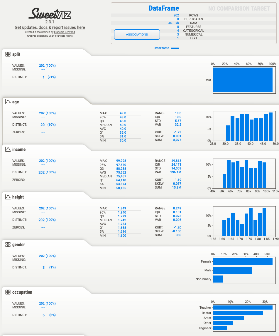
Now that we have things setup the first step in seeing a difference is through visualisations. The focus here being that by inspection of graphs and associated decriptitve statistics you can get an indication of whether things look similar or not.
Generating Automated Reports
- SweetViz is a nice package for generating all standard plots and descriptive statistics for our data.
- For the purpose of viewing basic plots for the data, there is little point in creating lots of custom functionality for this.
- Can consider custom functionality when things are right.
- Resources:
- For the purpose of viewing basic plots for the data, there is little point in creating lots of custom functionality for this.
In a few lines of code we can generate our plots
import sweetviz as sv

report_train = sv.analyze(
    data_processed[data_processed['split'] == 'train'],
    pairwise_analysis='off'
)

report_validation = sv.analyze(
    data_processed[data_processed['split'] == 'validation'],
    pairwise_analysis='off'
)

report_test = sv.analyze(
    data_processed[data_processed['split'] == 'test'],
    pairwise_analysis='off'
)

report_train.show_html('./data/train_report.html')
report_validation.show_html('./data/validation_report.html')
report_test.show_html('./data/test_report.html')
All things going well you should get output shown below:
Feature: registration_date                   |██████████| [100%]   00:00 -> (00:00 left)
Feature: registration_date                   |██████████| [100%]   00:00 -> (00:00 left)
Feature: registration_date                   |██████████| [100%]   00:00 -> (00:00 left)
Report ./data/train_report.html was generated! NOTEBOOK/COLAB USERS: the web browser MAY not pop up, regardless, the report IS saved in your notebook/colab files.
Report ./data/validation_report.html was generated! NOTEBOOK/COLAB USERS: the web browser MAY not pop up, regardless, the report IS saved in your notebook/colab files.
Report ./data/test_report.html was generated! NOTEBOOK/COLAB USERS: the web browser MAY not pop up, regardless, the report IS saved in your notebook/colab files.
Performing Statistical Tests and Calculating Custom Metrics
Approach to Perform This:
- Perform statistical testing and identify significant features after correcting for multiple tests.
- For the significant results, visualize the distributions using density plots.
- Assess the practical significance by examining the degree of separation between the distributions and the effect size (e.g., Cohen’s d).
- Conclude these are significantly different.
- Prioritize results that are both statistically significant and practically meaningful based on these factors.
- For results that are statistically significant but lack practical significance, interpret them cautiously or consider them less important.
Test Selection:
- Various different tests exist, so it’s worthwhile investigating their use based on data types and assumptions.
- Non-parametric tests might be a good candidate due to their lax constraints on the null hypothesis. These work well with continuous features.
- For example, a good candidate for direct distribution comparison would be the Kolmogorov-Smirnov test.
Possible Tests with Assumptions:
- Kruskal Wallis
- Assumptions: Independent samples, observations in split features are ordinal or continuous, distribution of features among limbs have the same shape (but not necessarily normal).
- Interpretations: Tests whether the medians of the groups are significantly different. It indicates that at least one group has a significantly different median compared to others.
- Mann Whitney U
- Assumptions: Independent samples, observations in groups are ordinal or continuous, distribution of features among splits have the same shape (but not necessarily normal).
- Interpretations: Tests whether the median between the two groups are significantly different. If the results are significant, then the medians show a significant difference.
- Kolmogorov-Smirnov
- Assumptions: Independent samples, distributions in groups are continuous.
- Interpretations: Compares the cumulative distribution functions (CDFs) of two groups and tests whether they are significantly different. If results are significant, this indicates the cumulative distributions are significantly different, hence the distributions are.
- Permutation
- Assumptions: Independent samples, observations in groups are ordinal or continuous.
- Interpretations: Tests the difference in means between groups by randomly permuting the group labels and calculating the test statistic for each permutation. If results are significant (within the extreme tails of the permutation distribution), it indicates that the difference in means between the two groups is significant.
- Chi-squared
- Assumptions: Independent samples, observations in groups are nominal or ordinal, frequency/count data, nominal/ordinal level of measurement, value of the expected cells should be 5 or more in at least 80% of the cells, and no cell should have an expected of less than one. Some empirical analysis on the suggested rules of thumbs might be overly conservative anyway.
- Interpretations: Tests if two categorical variables are independent or related by calculating the chi-square statistic on data. If results are significant (small p-value), there is a statistically significant relationship between the two variables; otherwise, not sufficient evidence to conclude the variables are related.
- Alongside performing testing, calculating an effect size measure can be important to help quantify the difference between distributions rather than if there is a difference or not, as spoken about here.
- There exists a number of standard measures that people tend to use. Cohen’s d is a good example that works with continuous features that follow a normal distribution.
- Due to this normal constraint (which a bunch of our features seem to violate) alongside susceptibility to outlier corruption, I decided to implement a new measure based on the following article, which shows a more robust yet somewhat consistent measure that can be used.
- Separate to hypothesis testing, other metrics can help measure divergence between probability distributions.
- A good example of this is Jensen-Shannon Divergence, which provides a normalized measure (0 implying identical and 1 implying maximally different) for difference.
- Didn’t come across any singular clear rule as to whether you should perform multiple-test corrections or not, it depends on the scenario
- In our case, it might not be needed but perhaps desirable since we might be making conclusions off the back of the results from multiple tests (whether each feature shows significant difference across splits) in the end in which case this is an advisable scenario.
- Some detailed discussion on whether it’s necessary and how to go about it can be found here.
- A breakdown of when to use which correction method is outlined here
- Multiple test correction helps account for FWER but there is a trade-off against power. For example, Bonferroni allows us to control FWER; however, it is known for being conservative on results and may vary depending on which tests are considered as part of the family.
- Even defining the familiy of tests can be subjective but can be influenced by a few key factors:
- The purpose of the tests: Tests that address a common research question or hypothesis should be grouped together as a family.
- The content of the tests: Tests that are similar in terms of the variables, hypotheses, and populations involved are more likely to be considered part of the same family.
- Current Implementation:
- For now, I have added corrections at a family = feature-test level:
- Reason for this is that we want to conclude whether for a given feature-test, that test suggests a significant difference between the various limbs we adjust across those limbs (4 choose 2 = 6 pairwise comparisons).
- The choice seems to also account for the research question (which features show differences, hence does a feature show a notable difference?) too since if we correct across feature-tests, we can be more confident as to whether a particular test shows a difference for a feature between groups.
- For now, I have added corrections at a family = feature-test level:
- Future Consideration:
- Perhaps making family = feature level might be good too?
- Since the tests being performed are similar in terms of hypothesis variables, then it could be considered part of the same family?
- Only issue is that different features could have different numbers of tests performed, so some might have different levels of corrections. This could adjust some features more than others, but perhaps this is okay?
- Perhaps making family = feature level might be good too?
- In general, it’s useful when you are performing rigorous planned testing rather than exploratory testing.
General Resources
- https://towardsdatascience.com/how-to-compare-two-or-more-distributions-9b06ee4d430b
- https://www.statisticshowto.com/probability-and-statistics/definitions/parametric-and-non-parametric-data/
- https://influentialpoints.com/Training/kolmogorov-smirnov-test-principles-properties-assumptions.htm
- https://influentialpoints.com/Training/wilcoxon-mann-whitney_principles-properties-assumptions.htm
- https://influentialpoints.com/Training/Kruskal-Wallis_ANOVA_use_and_misuse.htm
- https://www.ncbi.nlm.nih.gov/pmc/articles/PMC3900058/
- https://www.questionpro.com/blog/nominal-ordinal-interval-ratio-data/
- https://www.geo.fu-berlin.de/en/v/soga/ivy/Basics-of-Statistical-Hypothesis-Tests/Chi-Square-Tests/Chi-Square-Independence-Test/index.html
Below is some functionality that has been built to perform the majority of these tests, all you need to do is pass in the desired test you want to perform based on your use case. If you pass no specific tests in then the defaults would kick in which are sensible (chi squared test for discrete features and kolmogorov-smirnov and permutation tests for continuous features).
perform_pairwise_tests and dependencies
def cohens_d(group1, group2):
"""
Calculate Cohen's d effect size for two independent samples.
Cohen's d is a measure of standardized difference between two means.
It's commonly used to quantify the effect size in studies involving two independent groups.
Parameters
----------
group1 : pd.Series
List of values corresponding to the first sample.
group2 : pd.Series
List of values corresponding to the second sample.
Returns
-------
cohen_d : float
Cohen's d effect size measure.
effect_size_interpretation : str
Interpretation of effect size.
"""
# Calculate the sample size, mean & variance for both groups
n1, mean1, var1 = len(group1), np.mean(group1), group1.var(ddof=1)
n2, mean2, var2 = len(group2), np.mean(group2), group2.var(ddof=1)
# Calculate the pooled std
epsilon = 1e-6
pooled_std = np.sqrt(
(((n1 - 1) * var1 + (n2 - 1) * var2) / (n1 + n2 - 2)) + epsilon
)
cohen_d = (mean1 - mean2) / pooled_std
# Interpret the effect size
if abs(cohen_d) < 0.2:
effect_size_interpretation = "small"
elif abs(cohen_d) < 0.5:
effect_size_interpretation = "medium"
else:
effect_size_interpretation = "large"
return cohen_d, effect_size_interpretation
def aakinshin_effect_size(group1, group2, prob=0.2, num_quantiles=20):
"""
Calculate the Aakinshin effect size summary between our two groups.
Parameters
----------
group1 : pd.Series
First group of data.
group2 : pd.Series
Second group of data.
prob : float, optional
The probability defining the range for the shift function. Default is 0.2.
num_quantiles : int, optional
The number of quantiles to calculate. Default is 20.
Returns
-------
average_gamma : float
Average of the min & max gammas from your chosen gamma set.
gamma_effect_size : str
Interpretation of the effect size
detailed_gamma_distribution : dict
Dictionary of quantiles and corresponding gamma set.
Notes
-----
- The name of this function is based on the creator of the following blog post https://aakinshin.net/posts/nonparametric-effect-size/
which introduces the metric.
- The default choice of prob=0.2 is based on the articles as it captures the middle shifts and works well empirically.
- IQ Quantile Estimator is recommended https://aakinshin.net/posts/cs.msu-hd.quqntle/ but underflow errors were encountered so has been bypassed for now for more robust quantiles. Will be good to circle back
if time permits.
- scipy.stats.mstats contains some functions hdquantiles, hdmedian which were the ones tried but came across the error: FloatingPointError: underflow encountered in beta_ef associated with hdquantiles
"""
def pooled(x, y, func):
n_x = len(x)
n_y = len(y)
pooled_deviation = np.sqrt(
(((n_x - 1) * (func(x) ** 2)) + ((n_y - 1) * (func(y) ** 2))) / (n_x + n_y - 2)
)
return pooled_deviation
def hd_median(x):
return np.median(x)
def hd_median_absolute_deviation(x):
consistency_constant = 1.4826
sd_consistent_mad_estimator = (consistency_constant *
hd_median(np.abs(x - hd_median(x)))
)
return sd_consistent_mad_estimator
def pooled_hd_median_absolute_deviation(x, y):
return pooled(x, y, hd_median_absolute_deviation)
def gamma_effect_size(x, y, t):
Q_tx = mstats.mquantiles(x, prob=t)
Q_ty = mstats.mquantiles(y, prob=t)
pooled_deviation = pooled_hd_median_absolute_deviation(x, y)
# TODO: Is this the best way to handle division by 0???
if pooled_deviation == 0:
gamma_t = np.full_like(Q_tx, np.nan)
else:
gamma_t = (Q_ty - Q_tx) / pooled_hd_median_absolute_deviation(x, y)
return gamma_t
# Introducing set of all gammas
quantiles = np.linspace(prob, 1-prob, num_quantiles)
gammas = gamma_effect_size(group1, group2, quantiles)
# Calculating key metrics for our set of gammas
min_gamma = np.min(gammas)
max_gamma = np.max(gammas)
#range_gamma = max_gamma - min_gamma
# Single effect size score
average_gamma = (min_gamma + max_gamma) / 2
# All (quantile, gamma) pairs
detailed_gamma_distribution = {'quantiles': list(quantiles),
'gammas': list(gammas)}
# Interpret the effect size
if abs(average_gamma) < 0.2:
gamma_effect_size = "small"
elif abs(average_gamma) < 0.5:
gamma_effect_size = "medium"
else:
gamma_effect_size = "large"
return average_gamma, gamma_effect_size, detailed_gamma_distribution
def jensen_shannon_divergence(group1, group2, is_continuous=True):
"""
Calculate the Jensen-Shannon divergence between two groups for a given feature.
The Jensen-Shannon divergence is a symmetrized and smoothed version of the Kullback-Leibler divergence,
which measures the difference between two probability distributions. It is bound between 0 and 1, where
0 indicates identical distributions and 1 indicates maximally different distributions.
Parameters
----------
group1 : pd.Series
The first group's feature values.
group2 : pd.Series
The second group's feature values.
is_continous : bool
Flag for whether our distribution is continous or not.
If not then it is assumed to be discrete.
Returns
-------
jsd : float
Resulting JS-Divergence metric value.
Notes
-----
Stack post outlining ways to calculate: https://stackoverflow.com/questions/15880133/jensen-shannon-divergence
Other useful resources exist too:
https://arise.com/blogs/course/jensen-shannon-divergence/#:~:text=Jensen%20Shannon%20Divergence%20(JS%20Divergence,information%20represented%20by%20them%C2%A0distributions.
https://yongchaohuanghuchuan.github.io/2020-07-08-kl-divergence/
"""
group1 = group1.copy()
group2 = group2.copy()
if is_continuous:
# Define KDE estimation functions for groups
kde1 = gaussian_kde(group1)
kde2 = gaussian_kde(group2)
# Generate evaluation points for the KDE estimation
min_val = min(group1.min(), group2.min())
max_val = max(group1.max(), group2.max())
x_points = np.linspace(min_val, max_val, 1_000)
# Evaluate the PDF at the generated points
pdf1 = kde1.evaluate(x_points)
pdf2 = kde2.evaluate(x_points)
# Clipping the pdf distribution to remove underflow errors.
epsilon = 1e-10
pdf1 = np.clip(pdf1, epsilon, None)
pdf2 = np.clip(pdf2, epsilon, None)
# Normalize the PDFs
pdf1 /= pdf1.sum()
pdf2 /= pdf2.sum()
# Average the distributions
m = (pdf1 + pdf2) / 2
# Calculate the Jensen-Shannon divergence
jsd = 0.5 * (entropy(pdf1, m) + entropy(pdf2, m))
else:
# Getting the probability distributions
pmf1 = group1.value_counts(normalize=True)
pmf2 = group2.value_counts(normalize=True)
# Find the union of unique values in pmf1 and pmf2
unique_values = np.union1d(pmf1.index, pmf2.index)
# Adjust the probability distributions to account for this
pmf1 = pmf1.reindex(unique_values, fill_value=0)
pmf2 = pmf2.reindex(unique_values, fill_value=0)
# Average the distributions
m = (pmf1 + pmf2) / 2
# Calculate the Jensen-Shannon divergence
jsd = 0.5 * (entropy(pmf1, m) + entropy(pmf2, m))
return jsd
def kruskal_wallis_test(group1, group2):
"""
Perform Kruskal Wallis test to compare the distributions of two groups.
Parameters
----------
group1 : array-like
The first group of observations.
group2 : array-like
The second group of observations.
Returns
-------
test_statistic : float
The Kruskal-Wallis H statistic.
p_value : float
The p-value associated with the test.
"""
test_statistic, p_value = kruskal(group1, group2)
return test_statistic, p_value
def mann_whitney_u_test(group1, group2):
"""
Perform the Mann-Whitney U test to compare the distributions of two independent groups.
Parameters
----------
group1 : array-like
The first group of observations.
group2 : array-like
The second group of observations.
Returns
-------
test_statistic : float
The Mann-Whitney U statistic.
p_value : float
The p-value associated with the test.
"""
test_statistic, p_value = mannwhitneyu(group1, group2, alternative="two-sided")
return test_statistic, p_value
def kolmogorov_smirnov_test(group1, group2):
"""
Perform the Kolmogorov Smirnov test to compare the distributions of two independent groups.
Parameters
----------
group1 : array-like
The first group of observations.
group2 : array-like
The second group of observations.
Returns
-------
test_statistic : float
The Kolmogorov Smirnov statistic.
p_value : float
The p-value associated with the test.
"""
test_statistic, p_value = ks_2samp(group1, group2)
return test_statistic, p_value
def aggregated_low_counts(contingency):
"""
Aggregate up all observed frequencies for corresponding expected frequencies that are less than 5.
Parameters
----------
contingency : pd.DataFrame
Input contingency table containing feature values by groups.
Returns
-------
contingency : pd.DataFrame
Output contingency table containing aggregated results.
Notes
-----
Most resources either don't talk about handling cases where the expected values are less than 5 or if they do they suggest using another test.
Here is a few which suggest aggregating seem plausible: http://community.jmp.com/t5/Discussions/How-can-I-do-a-chi-square-test-when-20-of-the-cells-that-have-an/td-p/38928,
https://ondata.blog/articles/implications-scikit-learn-21455/
"""
# Creating data copy
contingency = contingency.copy()
# Calculate expected contingency
expected = np.outer(contingency.sum(axis=1),
contingency.sum(axis=0)) / contingency.sum().sum()
while (expected < 5).any():
# Find row with the smallest sum
row1_min = contingency.sum(axis=1).idxmin()
# Find the row with 2nd smallest sum
row2_min = contingency.drop(row1_min).sum(axis=1).idxmin()
# Combine the rows by summing them
new_row = contingency.loc[row1_min, :] + contingency.loc[row2_min, :]
# Drop the old rows and add new one
contingency = contingency.drop([row1_min, row2_min])
contingency.loc["Combined_" + str(row1_min) + "_" + str(row2_min)] = new_row
# Recalculate the expected frequencies
expected = np.outer(contingency.sum(axis=1),
contingency.sum(axis=0)) / contingency.sum().sum()
return contingency
def chi_squared_test(feature, groups):
"""
Perform the chi-squared independence test to compare discrete
distributions of two groups.
Parameters
----------
feature : array-like
The feature observations across groups.
groups : array-like
The group name data for each feature value.
Returns
-------
test_statistic : float
The Chi-Squared test statistic.
p_value : float
The p-value associated with the test.
Notes
-----
The following article provides more detailed notes on how chi squared is working:
https://www.geo.fu-berlin.de/en/v/soga-py/Basics-of-statistics/Hypothesis-Tests/Chi-Square-Tests/Chi-Square-Independence-Test/index.html
"""
# Convert inputs to 1D arrays if they're pandas Series
if isinstance(feature, pd.Series):
feature = feature.squeeze()
if isinstance(groups, pd.Series):
groups = groups.squeeze()
# If still multidimensional, take first column
if isinstance(feature, pd.DataFrame):
feature = feature.iloc[:, 0]
if isinstance(groups, pd.DataFrame):
groups = groups.iloc[:, 0]
contingency_table = pd.crosstab(
feature, groups
)
if contingency_table.size == 0:
print("Contingency table is empty. Chi-squared test cannot be performed.")
return None, None
# Aggregating results if less than 5.
contingency_table = aggregated_low_counts(contingency_table)
test_statistic, p_value, _, _ = chi2_contingency(contingency_table)
return test_statistic, p_value
def permutation_test(group1, group2, n_permutations=2000):
"""
Perform a permutation test to compare the means of two independent groups.
Parameters
----------
group1 : array-like
The first group of observations.
group2 : array-like
The second group of observations.
n_permutations : int, optional
The number of permutations to perform (default is 2000).
Returns
-------
p_value : float
The p-value associated with the test.
"""
# Convert to numpy arrays & combine data
group1 = np.array(group1)
group2 = np.array(group2)
combined_data = np.concatenate((group1, group2))
# Calculate true observed mean difference
observed_diff_mean = np.mean(group1) - np.mean(group2)
# Loop over, shuffle, calculate and then list difference in mean of permuted samples
permuted_diffs = []
for _ in range(n_permutations):
permuted_data = np.random.permutation(combined_data)
perm_group1 = permuted_data[:len(group1)]
perm_group2 = permuted_data[:len(group2)]
permuted_diff_mean = np.mean(perm_group1) - np.mean(perm_group2)
permuted_diffs.append(permuted_diff_mean)
# Convert to array and calculate p_value statistic
permuted_diffs = np.array(permuted_diffs)
p_value = (
np.sum(np.abs(permuted_diffs) >= np.abs(observed_diff_mean)) / n_permutations
)
test_statistic = None
return test_statistic, p_value
def apply_test_corrections(results_df, correction_method="bonferroni", fwer=0.05):
"""
Apply multiple comparison corrections to the p-values in the results data.
Parameters
----------
results_df : pd.DataFrame
Dataframe containing the test results for each pair of groups (per feature) and each test function.
correction_method : str, optional
Multiple test correction method to apply ('bonferroni', 'sidak', etc). Default is 'bonferroni'.
fwer : float
Family wise error rate, or the probability of at least 1 type I error across your family of hypothesis tests.
Returns
-------
results_df : pd.DataFrame
Dataframe with additional columns for corrected p-values and significance.
"""
features = results_df["feature"].unique()
test_names = results_df["test_name"].unique()
for feature in features:
for test_name in test_names:
feature_test_mask = (results_df["feature"] == feature) & (
results_df["test_name"] == test_name
)
p_values = results_df.loc[feature_test_mask, "p_value"].to_numpy()
if np.isnan(p_values).all():
# Handle case when p-values are null
# significant_results = np.full(len(p_values), False)
# corrected_p_values = np.full(len(p_values), np.nan)
significant_results = pd.Series(
False, index=results_df.index[feature_test_mask], dtype=bool
)
corrected_p_values = pd.Series(
np.nan, index=results_df.index[feature_test_mask], dtype=float
)
else:
# Remove NaN values from p values before applying.
valid_p_values_mask = ~np.isnan(p_values)
valid_p_values = p_values[valid_p_values_mask]
valid_indices = results_df.index[feature_test_mask][
valid_p_values_mask
]
significant_results_array, corrected_p_values_array, _, _ = (
multipletests(
valid_p_values,
alpha=fwer,
method=correction_method,
returnsorted=False,
)
)
significant_results = pd.Series(
significant_results_array, index=valid_indices, dtype=bool
)
corrected_p_values = pd.Series(
corrected_p_values_array, index=valid_indices, dtype=float
)
# Adding adjusted p_value along with significant or not
results_df.loc[feature_test_mask, f"significant_{correction_method}"] = (
significant_results
)
results_df.loc[
feature_test_mask, f"{correction_method}_corrected_p_value"
] = corrected_p_values
return results_df
def perform_pairwise_tests(
df,
discrete_cols=None,
continuous_cols=None,
group_col="split",
test_functions={
"discrete": [chi_squared_test],
"continuous": [kolmogorov_smirnov_test, permutation_test],
},
fwer=0.05,
):
"""
Compare the distributions of the specified columns across multiple groups in a pandas dataframe.
Parameters
----------
df : pandas.DataFrame
The input dataframe.
discrete_cols : list
A list of discrete column names to compare.
continuous_cols : list
A list of continuous column names to compare.
group_col : str
The name of the column that defines the groups.
test_functions : dict
A dictionary mapping column types to a list of test functions.
fwer : float
Family wise error rate, or the probability of at least 1 type I error across your family of hypothesis tests.
Returns
-------
pandas.DataFrame
A dataframe containing the test statistic and p-value for each column and group comparison.
"""
# Get the unique group values
groups = df[group_col].unique()
# Storing our test results
results = []
# Iterate over the discrete columns
if discrete_cols:
for col in discrete_cols:
for group1, group2 in itertools.combinations(groups, 2):
# Filter the dataframe to get the data for the two groups
df_group1 = df[df[group_col] == group1][col]
df_group2 = df[df[group_col] == group2][col]
for test_func in test_functions['discrete']:
if test_func.__name__ == 'chi_squared_test':
# Data format specific for chi-squared test.
chi_squared_data = df.loc[df[group_col].isin([group1, group2]), [col, group_col]]
test_statistic, p_value = test_func(chi_squared_data[col], chi_squared_data[group_col])
else:
test_statistic, p_value = test_func(df_group1, df_group2)
jsd = jensen_shannon_divergence(
df_group1, df_group2, is_continuous=False
)
results.append(
{
"feature": col,
"group1": group1,
"group2": group2,
"test_name": test_func.__name__,
"test_statistic": test_statistic,
"p_value": p_value,
"type": "discrete",
"js_divergence": jsd,
"cohens_d": np.nan,
"aakinshin_gamma": np.nan,
"aakinshin_gamma_dist": np.nan,
"effect_size": None,
}
)
# Iterate over the continuous columns
if continuous_cols:
for col in continuous_cols:
for group1, group2 in itertools.combinations(groups, 2):
# Filter the dataframe to get the data for the two groups
df_group1 = df[df[group_col] == group1][col]
df_group2 = df[df[group_col] == group2][col]
for test_func in test_functions["continuous"]:
test_statistic, p_value = test_func(df_group1, df_group2)
jsd = jensen_shannon_divergence(
df_group1, df_group2, is_continuous=True
)
cohen_d, _ = cohens_d(df_group1, df_group2)
(avg_aakinshin_effect_size,
aakinshin_effect_size_interpretation,
full_aakinshin_effect_dist) = aakinshin_effect_size(df_group1, df_group2)
results.append(
{
"feature": col,
"group1": group1,
"group2": group2,
"test_name": test_func.__name__,
"test_statistic": test_statistic,
"p_value": p_value,
"type": "continuous",
"js_divergence": jsd,
"cohens_d": cohen_d,
"aakinshin_gamma": avg_aakinshin_effect_size,
"aakinshin_gamma_dist": full_aakinshin_effect_dist,
"effect_size": aakinshin_effect_size_interpretation,
}
)
# Create the dataframe with the results
result_df = pd.DataFrame(results)
# Apply multiple test corrections
result_df = apply_test_corrections(result_df, fwer=fwer)
return result_df
hypothesis_testing_results = perform_pairwise_tests(
    data_processed,
    discrete_cols = config['data_types']['features']['discrete'],
    continuous_cols = config['data_types']['features']['continuous'],
    group_col = 'split'
)
hypothesis_testing_results
Which gives you something like:
feature	group1	group2	test_name	test_statistic	p_value	type	js_divergence	cohens_d	aakinshin_gamma	aakinshin_gamma_dist	effect_size	significant_bonferroni	bonferroni_corrected_p_value
0	gender	train	test	chi_squared_test	24.517898	4.742486e-06	discrete	0.019733	NaN	NaN	NaN	None	True	1.422746e-05
1	gender	train	validation	chi_squared_test	0.502874	7.776825e-01	discrete	0.000676	NaN	NaN	NaN	None	False	1.000000e+00
2	gender	test	validation	chi_squared_test	9.136032	1.037853e-02	discrete	0.016459	NaN	NaN	NaN	None	True	3.113559e-02
12	age	train	test	kolmogorov_smirnov_test	0.760000	4.981798e-90	continuous	0.444449	-2.701849	2.066277	{'quantiles': [0.2, 0.23157894736842108, 0.263...]}	large	True	1.494539e-89
13	age	train	test	permutation_test	NaN	0.000000e+00	continuous	0.444449	-2.701849	2.066277	{'quantiles': [0.2, 0.23157894736842108, 0.263...]}	large	True	0.000000e+00
14	age	train	validation	kolmogorov_smirnov_test	1.000000	6.254039e-135	continuous	0.692191	-6.079607	5.024814	{'quantiles': [0.2, 0.23157894736842108, 0.263...]}	large	True	1.876212e-134
- Now the tests just performed act in a pairwise fashion between data splits.
- Performing tests at a higher level (not pairwise between all combinations but instead feeding the featurea across each split).
- I suspect this might be the better way to perform the chi2 test (not pairwise but across all splits at once) as it aligns with the level at which we ultimately want to perform conclusions (is feature different across splits rather than a specific difference between a given split pair).
- These are not accounting for multiple tests but should be okay since exploratory and chi2 is conservative as is.
- Usage:
- These should be used in conjunction with the pairwise tests, plots, and other factors to gauge whether things are lining up.
Non-Pairwise tests: Continuous Features
Here we make use of “one-way ANOVA” to test the null hypothesis that our data splits have the same population mean.
perform_continuous_feature_test
    from scipy.stats import f_oneway
    def perform_continuous_feature_test(data, features,
    significance_level=0.05, split_column="split"):
        """Perform significance test between continuous distributions and store the results in a DataFrame.

        Parameters
        ----------
        data : pandas.DataFrame
            The input data.
        features : list
            A list of feature columns to test.
        significance_level : float, optional
            The significance level for the test, by default 0.05.
        split_column : str, optional
            The column name containing the limb information, by default "split".

        Returns
        -------
        pandas.DataFrame
            A DataFrame containing the test results for each feature.

        Examples
        --------
        >>> continuous_features = ['age', 'income', 'purchase_amount']
        >>> results_df = perform_continuous_feature_test_to_df(data, continuous_features)
        """
        results = []
        for feature in features:
            limbs = data[split_column].unique()
            feature_values = [data[data[split_column] == limb][feature] for limb in limbs]

            f_statistic, p_value = f_oneway(*feature_values)

            result = {
                'feature': feature,
                'f_statistic': f_statistic,
                'p_value': p_value,
                'significant': p_value < significance_level
            }
            results.append(result)
perform_continuous_feature_test(
    data_processed,
    list(config["data_types"]["features"]["continuous"].keys()),
    split_column='split'
)
This gives output like the following:
feature	f_statistic	p_value	significant
0	age	1888.160614	0.000000e+00	True
1	income	3625.717099	0.000000e+00	True
2	height	509.976783	2.874950e-153	True
Pairwise tests: Discrete Features
Likewise we can use the chi squared test for discrete features. Again this is operating at an aggregated level.
perform_categorical_feature_test
    import pandas as pd
    from scipy.stats import chi2_contingency
    def perform_categorical_feature_test(data, features, significance_level=0.05, split_column="split"):
        """Perform significance test between discrete distributions and store the results in a DataFrame.

        Parameters
        ----------
        data : pandas.DataFrame
            The input data.
        features : list
            A list of feature columns to test.
        significance_level : float, optional
            The significance level for the test, by default 0.05.
        split_column : str, optional
            The column name containing the limb information, by default "split".

        Returns
        -------
        pandas.DataFrame
            A DataFrame containing the test results for each feature.

        Examples
        --------
        >>> categorical_features = ['gender', 'region']
        >>> results_df = perform_categorical_feature_test_to_df(data, categorical_features)
        """
        results = []
        for feature in features:
            contingency_table = pd.crosstab(data[feature], data[split_column])

            chi2_statistic, p_value, _, _ = chi2_contingency(contingency_table)

            result = {
                'feature': feature,
                'chi2_statistic': chi2_statistic,
                'p_value': p_value,
                'significant': p_value < significance_level
            }
            results.append(result)

        return pd.DataFrame(results)
perform_categorical_feature_test(
    data_processed,
    list(config["data_types"]["features"]["discrete"].keys()),
    split_column='split'
)
Which gives:
	feature	chi2_statistic	p_value	significant
0	gender	25.201433	4.582897e-05	True
1	occupation	74.951330	5.044603e-13	True
2	owns_car	90.128987	2.683733e-20	True
3	registration_date	2000.000000	2.344813e-24	True
Custom Visualisations for Significant Features
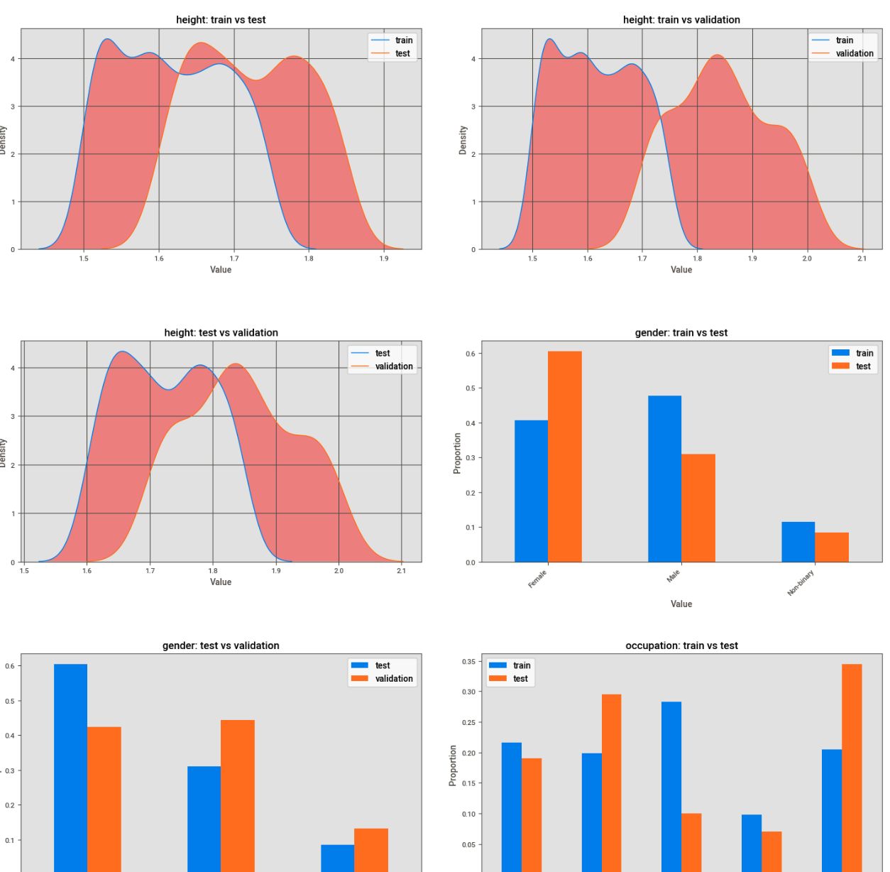
In a prior section we already performed visualisations so you might be wondering what the point of this section is. The way I see it is the initial visualisations were more generic with a purpose of getting a feel for the features by inspection. However now that we have explored and have a grip on which features or significant vs not we can generate more custom plots to confirm these for those we deem as significant.
Plotting Distributions of “Statistically Significant” Features
- Purpose:
- Plotting those significant feature distributions to help grasp their practical significance.
Continuous Features
- Density Plots:
- Density plots can help assess practical significance by visualizing the distributions across the various pairs of limbs.
- If the distributions overlap substantially, even if they are statistically significant, the practical difference may be negligible. Conversely, if the distributions are well separated, it may indicate a practical difference even if the statistical difference is marginal due to small sample size.
- A red color has been added to regions in the plot which signifies no overlap between the two distributions. This can help visually flesh out the amount of difference between them.
Discrete Features
- Bar Charts:
- Grouped bar charts are perhaps the best visualizations to use for discrete data and the recommended go-to.
- The bars for each group are positioned side-by-side, allowing for easy comparison of the values between the two groups across the different categories.
- Designed for when you want to compare values between two or more groups across multiple categories.
- Stacked bar charts can be challenging to interpret precisely, especially for the lower segments. They are best used when the main goal is to show the overall trend and composition, not to make exact comparisons between subcategories.
- Grouped bar charts are perhaps the best visualizations to use for discrete data and the recommended go-to.
plot_significant_features
    def plot_significant_features(data_df, results_df, significance_col="significant_bonferroni"):
        """
        Generate plots for features with significant differences between groups.
        """
        # Filter for significant results and remove duplicate tests for same feature-group pairs
        significant_results = results_df[results_df[significance_col] == True]

        # For continuous features, keep only one test type (kolmogorov_smirnov_test)
        continuous_results = significant_results[
            (significant_results['type'] == 'continuous') &
            (significant_results['test_name'] == 'kolmogorov_smirnov_test')
        ]

        # Get discrete results
        discrete_results = significant_results[significant_results['type'] == 'discrete']

        # Combine and get unique feature-group combinations
        unique_results = pd.concat([continuous_results, discrete_results])
        unique_results = unique_results.drop_duplicates(subset=['feature', 'group1', 'group2'])

        # Instead of iterating on unique_results.iterrows(), reset the index
        unique_results = unique_results.reset_index(drop=True)

        # Check if there are any significant results
        if len(unique_results) == 0:
            print("No significant features found to plot")
            return

        # Calculate improved grid dimensions
        n_plots = len(unique_results)
        n_cols = 2  # Fix number of columns to 2
        n_rows = (n_plots + 1) // 2  # Ensure we round up when dividing

        # Create figure and axes with updated dimensions
        fig, axes = plt.subplots(n_rows, n_cols, figsize=(15, 5 * n_rows), squeeze=False)

        # Rest of the plotting code remains the same
        for i, row in unique_results.iterrows():
            row_idx = i // n_cols
            col_idx = i % n_cols

            feature = row['feature']
            group1 = row['group1']
            group2 = row['group2']
            feature_type = row['type']

            # Configure subplot
            ax = axes[row_idx, col_idx]
            ax.set_facecolor("#e5e5e5")
            ax.grid(True)

            # Get data for both groups
            group1_data = data_df[data_df["split"] == group1][feature]
            group2_data = data_df[data_df["split"] == group2][feature]

            if feature_type == "continuous":
                # Plot density plots for continuous features
                sns.kdeplot(data=group1_data, label=group1, ax=ax, linewidth=1)
                sns.kdeplot(data=group2_data, label=group2, ax=ax, linewidth=1)

                # Highlight non-overlapping regions
                x1, y1 = ax.lines[0].get_data()
                x2, y2 = ax.lines[1].get_data()
                x_common = np.linspace(min(x1.min(), x2.min()), max(x1.max(), x2.max()), 1000)
                y1_interp = np.interp(x_common, x1, y1)
                y2_interp = np.interp(x_common, x2, y2)

                ax.fill_between(x_common, y1_interp, y2_interp,
                            where=(y1_interp > y2_interp),
                            facecolor="red", alpha=0.4)
                ax.fill_between(x_common, y1_interp, y2_interp,
                            where=(y2_interp > y1_interp),
                            facecolor="red", alpha=0.4)

            else:  # Discrete features
                # Calculate proportions for discrete features
                props1 = group1_data.value_counts(normalize=True)
                props2 = group2_data.value_counts(normalize=True)

                # Create DataFrame for plotting
                plot_df = pd.DataFrame({
                    group1: props1,
                    group2: props2
                }).fillna(0)

                # Plot bar chart
                plot_df.plot(kind='bar', ax=ax)

                # Rotate x-axis labels
                ax.set_xticklabels(plot_df.index, rotation=45, ha='right')

            # Set titles and labels
            ax.set_title(f"{feature}: {group1} vs {group2}")
            ax.set_xlabel("Value")
            ax.set_ylabel("Density" if feature_type == "continuous" else "Proportion")
            ax.legend()

        # Remove empty subplots
        for idx in range(n_plots, n_rows * n_cols):
            row = idx // n_cols
            col = idx % n_cols
            fig.delaxes(axes[row, col])

        plt.tight_layout()  # Add tight_layout to prevent overlapping
        plt.show()
plot_significant_features(
    data_processed,
    hypothesis_testing_results,
    significance_col="significant_bonferroni"
)
The output plots look something like below where both continuous and discrete features are displayed within the same figure. The red portion in the continuous plots represents the area in-between the curves, this helps highlight the magnitude of the differences giving us a better immediate sense of “how” different the features are.
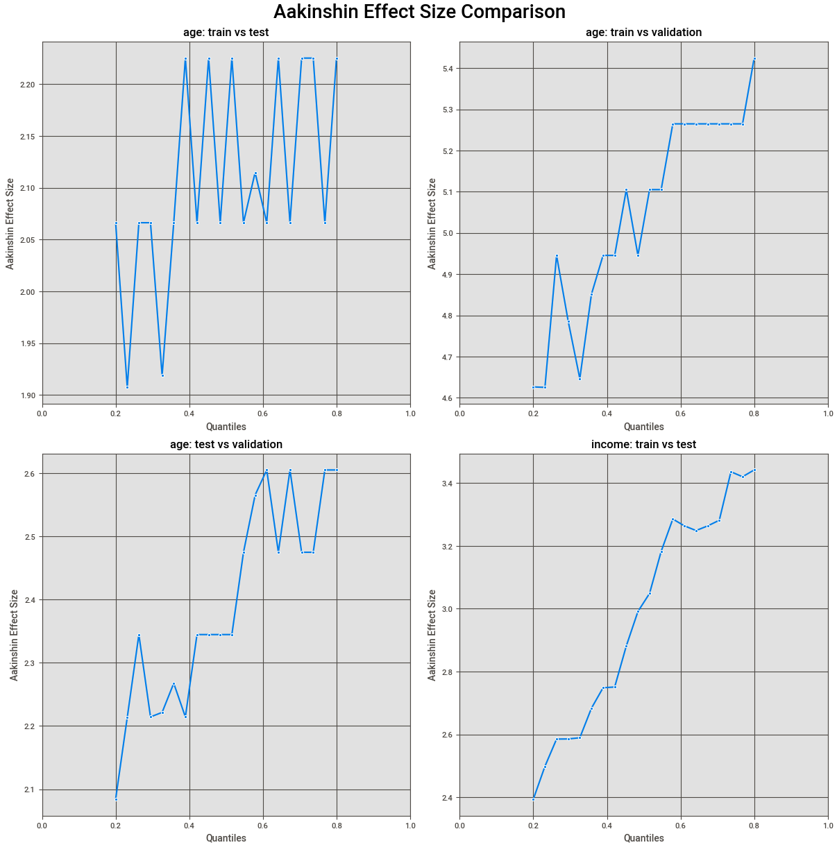
Plotting Effect Sizes for Continuous “Statistically Significant” Features
- A single value for effect size might not summarize things well, especially for complex distributions, and thus it’s useful to view plots where appropriate. The following are key considerations:
Observations
- Edge Cases:
- Edge cases are possible where the median value is 0 for features, which can cause the pooled estimates to be 0, leading to zero-division errors.
- This, in general, can occur if at least 50% of your data equals the 2nd or 0.5 quantile.
- For now, these have been avoided, and the corresponding plots have been left blank, but more techniques can handle this which haven’t been implemented yet.
- Interpretation Notes:
- The order in which the two groups were compared matters, and if they were reversed, the graph would be reflected in the x-axis.
- The magnitude of the effect size is important as it can tell you for a given quantile of the distributions what the scale of difference was.
- If values fluctuate close to zero across all quantiles, it suggests the actual differences are likely very small and practically insignificant, meaning differences flagged as statistically significant likely arose due to large sample sizes.
- With a large enough sample, even trivial differences can become statistically significant.
- On the contrary, very large effect size differences across quantiles could indicate practical differences.
plot_significant_effect_sizes
    def plot_significant_effect_sizes(results_df, significance_col='significant_bonferroni'):
        """
        Generate plots showing effect sizes for significant features.
        """
        # Filter for significant continuous features with KS test only
        significant_results = results_df[
            (results_df[significance_col] == True) &
            (results_df['type'] == 'continuous') &
            (results_df['test_name'] == 'kolmogorov_smirnov_test')
        ]

        unique_results = significant_results.drop_duplicates(subset=['feature', 'group1', 'group2'])

        # Early return if no results
        if len(unique_results) == 0:
            print("No significant continuous features found")
            return

        # Plot setup with better grid calculation
        n_plots = len(unique_results)
        n_cols = min(2, n_plots)  # Max 2 columns
        n_rows = (n_plots + (n_cols - 1)) // n_cols

        # Create figure and axes
        fig, axes = plt.subplots(
            n_rows, n_cols,
            figsize=(12, 6 * n_rows),
            squeeze=False,
            constrained_layout=True
        )

        # Set title
        fig.suptitle("Aakinshin Effect Size Comparison", fontsize=20)

        # Configure all subplots
        for row in range(n_rows):
            for col in range(n_cols):
                axes[row, col].set_facecolor("#e5e5e5")
                axes[row, col].grid(True)

        # Plot each feature
        for idx, row in enumerate(unique_results.itertuples()):
            row_idx = idx // n_cols
            col_idx = idx % n_cols

            # Safety check for index bounds
            if row_idx >= n_rows or col_idx >= n_cols:
                continue

            # Extract effect distribution
            effect_dist = row.aakinshin_gamma_dist
            if isinstance(effect_dist, str):
                effect_dist = eval(effect_dist)

            # Create effect size DataFrame
            effect_df = pd.DataFrame(effect_dist)

            # Plot effect size distribution
            ax = axes[row_idx, col_idx]
            sns.lineplot(
                data=effect_df,
                x='quantiles',
                y='gammas',
                marker='o',
                ax=ax
            )

            # Configure plot
            ax.set_xlim(0, 1)
            ax.set_title(f"{row.feature}: {row.group1} vs {row.group2}")
            ax.set_xlabel("Quantiles")
            ax.set_ylabel("Aakinshin Effect Size")

            # Add note for NaN values
            if np.all(np.isnan(effect_df["gammas"].values)):
                ax.text(
                    0.5, 0.5,
                    'All gammas are NaN (PMAD=0)',
                    transform=ax.transAxes,
                    ha='center',
                    va='center',
                    fontsize=12
                )

        # Remove empty subplots
        for idx in range(n_plots, n_rows * n_cols):
            row_idx = idx // n_cols
            col_idx = idx % n_cols
            fig.delaxes(axes[row_idx, col_idx])

        plt.show()
plot_significant_effect_sizes(
    hypothesis_testing_results,
    significance_col="significant_bonferroni"
)
The results look something like:
Making Conclusions
- Summary of Findings:
- Taking into account our various datapoints (summary statistics, distribution plots, statistical tests, effect size measures & other metrics), it seems like the distributions of features amongst the splits for our data are showing signs of significant difference.
- Large differences are visible and most if not all tests show a significant result, the magnitude of the difference across the various tests seems large enough to suggest a true practical significant difference.
- Taking into account our various datapoints (summary statistics, distribution plots, statistical tests, effect size measures & other metrics), it seems like the distributions of features amongst the splits for our data are showing signs of significant difference.
- Ranking of Features:
- Below is a ranking of the features based on which seem to show the most difference.
- The lower the rank number (e.g., rank = 1) means more difference, and the higher the rank (e.g., rank = 10) means less difference.
- This is done by aggregating the testing results/measures each feature shows across the various pairwise limb comparisons and then using these to create a ranking based on which shows the most difference.
- In case you want to stratify or investigate certain features in more detail, this can provide some guidance.
- Below is a ranking of the features based on which seem to show the most difference.
rank_features
    def rank_features(results_table,
                 significance_column='significant_bonferroni',
                 continuous_test='kolmogorov_smirnov_test'):
        """
        Rank features based on which show the most signs of difference.

        Parameters
        ----------
        results_table : pd.DataFrame
            One single results table containing all metrics and statistical test results for features.
        significance_column : str
            Name of the column which tells us about the significance
        continuous_test : str
            Name of the statistical test that we want to use as part of ranking

        Returns
        -------
        feature_ranks : pd.DataFrame
            Final dataframe containing the features and their rankings.

        Notes
        -----
        ...
        """
        results_table = results_table.copy()

        # Mapping significance column to 1's and 0's for downstream summation
        results_table[significance_column] = results_table[significance_column].map({True: 1, False: 0})

        # Filtering our testing to remove duplicates and only keep a single test results
        if continuous_test == 'kolmogorov_smirnov_test':
            results_table = results_table[
                (results_table['type'] == 'discrete') | ((results_table['type'] == 'continuous') & (results_table['test_name'] == 'kolmogorov_smirnov_test'))
            ]
        elif continuous_test == 'permutation_test':
            results_table = results_table[
                (results_table['type'] == 'discrete') | ((results_table['type'] == 'continuous') & (results_table['test_name'] == 'permutation_test'))
            ]

        elif continuous_test == 'both':
            # For features if running multiple tests as we are using the whole results table, this might throwan off calcuations due to multiple
            # entries for the same feature.
            pass

        # Grouping features and calculating their ovral divergence score and significant results count
        feature_scores = results_table.groupby('feature').agg({
            'js_divergence': 'sum',
            significance_column: 'sum'
        }).reset_index()

        # Combining the different scores to calculate a single measure which can be used
        feature_scores['feature_rank'] = (
            feature_scores['js_divergence'].rank(method='dense', ascending=False) +
            feature_scores[significance_column].rank(method='dense', ascending=False)
        )

        # Sorting and returing final dataframe
        feature_ranks = feature_scores[['feature', 'feature_rank']].sort_values('feature_rank').reset_index(drop=True)
        feature_ranks['feature_rank'] = feature_ranks['feature_rank'].rank(method='dense').astype(int)

        return feature_ranks
ranked_feature_differences = utils.rank_features(
    hypothesis_testing_results,
    significance_column="significant_bonferroni",
    continuous_test="kolmogorov_smirnov",
)
ranked_feature_differences
This gives a view like:
	feature	feature_rank
0	income	1
1	age	2
2	height	3
3	registration_date	3
4	owns_car	4
5	occupation	5
6	gender	6