Autoencoders Explained - Breathing Life into Data

Nish · August 2, 2023

Intro   NLP   AI   Autoencoders

Table of Contents

• What are Autoencoders?
  • Autocoder Architecture
  • What makes these models generative?
• What does coding up an autoencoder look like?
  • Setting Parameters and Importing
  • Load & Preprocessing Data
  • The Encoder
  • The Decoder
  • Autoencoder
  • Training
• Drawbacks of standard autoencoders
• Resolving Autoencoder Problem: Introducing the Variational Autoencoder (VAE)
  • Maths: Normal Distribution + KL divergence loss
  • Coding up a VAE
• Real World Usecases
• Resources

What are Autoencoders?

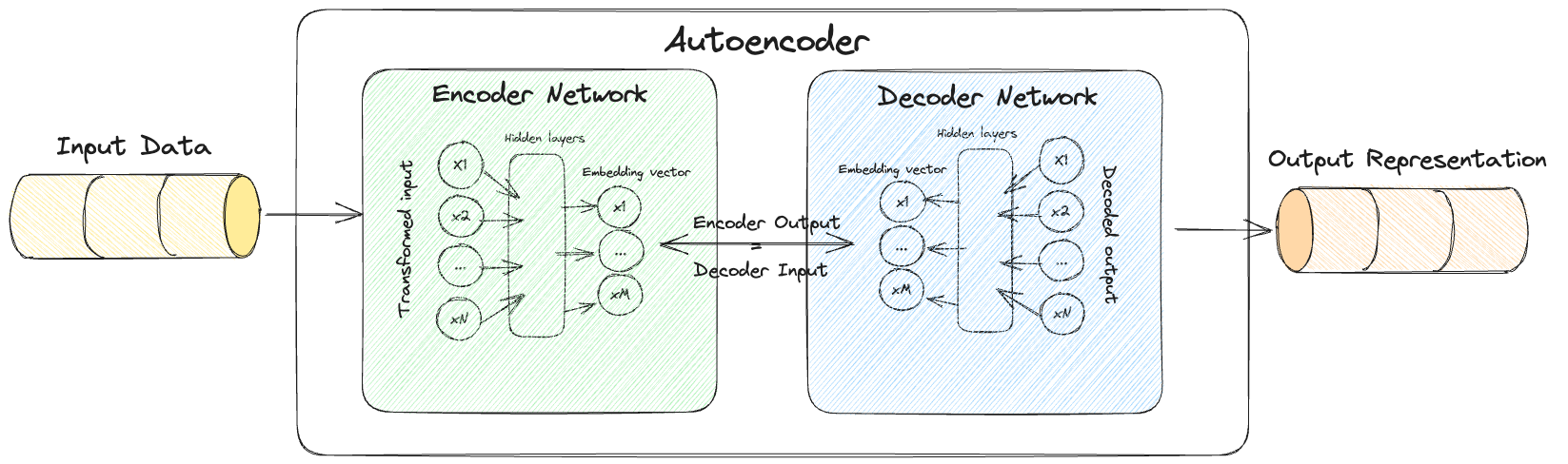
Autoencoders can be thought of as a type of model which are able to compress input data into a latent space and then reconstruct original esque data from this learned compressed representation. This can be used for generative tasks aswell as other types of non-generative tasks depending on the end design.

Autocoder Architecture

They consist of two parts

1. Encoder
   • A neural network that compresses high-dimensional input data (could be images, text, audio etc) into a lower dimensional embedding vector.
2. Decoder
   • A neural network that decompresses a given embedding vector (output of the encoder) back to the original domain (could be images, text, audio etc).

These two parts can then be combined together into a “single model” which then makes up the autoencoder (checkout the illustration below).

High level view of the underlying architecture of autocoder models

What makes these models generative?

At it’s core generative models are those which can learn from a given dataset (observations) a distribution $P_{\text{model}}$ that mimics the underlying distribution of the data $P_{\text{data}}$. By then sampling from this learned distribution $P_{\text{model}}$ it can generate new data which appears like it has been taken from the original data distribution $P_{\text{data}}$.

In our case when training the model $P_{\text{model}}$ would be the learned latent space of embedding vectors which you could then sample from to generate new items.

What does coding up an autoencoder look like?

For demo purposes I will create an autoencoder which works with an image dataset of greyscale images (28x28 pixels). We will make use of the TensorFlow framework, in particular it’s functional API. The code here draws heavily on Generative Deep Learning so be sure to check it out, great resource!

Note: The general model architecture provided can be used regardless of what the data is. The main thing to bear in mind would be to alter the shape of the input and output tensors (along with network parameters) based on the requirements of your dataset.

Setting Parameters and Importing

We start by importing the relevant libraries. I decided to just important the base TensorFlow library maintaining any particular classes used inside the code snippets themselves for easier referencing.

import tensorflow as tf

IMAGE_SIZE = 32
CHANNELS = 1
BATCH_SIZE = 100
BUFFER_SIZE = 1000
VALIDATION_SPLIT = 0.2
EMBEDDING_DIM = 2
EPOCHS = 10

Load & Preprocessing Data

Since we are using the Fashion MNIST dataset as our dataset it’s important that we process the image first.

# Load the data
(x_train, y_train), (x_test, y_test) = tf.keras.datasets.fashion_mnist.load_data()

def img_preprocessing(imgs):
    """
    Normalize and reshape the images

    Parameters
    ----------
    imgs: np.ndarray
        Numpy array of image pixel values.
    
    Returns
    -------
    imgs: np.ndarray
        Numpy array of image pixel values after preprocessing has been applied.
    """
    
    imgs = imgs.astype("float32") / 255.0
    imgs = np.pad(imgs, ((0, 0), (2, 2), (2, 2)), constant_values=0.0)
    imgs = np.expand_dims(imgs, -1)
    
    return imgs

# Applying preprocessing to our data
x_train = img_preprocessing(x_train)
x_test = img_preprocessing(x_test)

Here’s what each line in the function does:

• imgs = imgs.astype("float32") / 255.0:
  • This line changes the datatype of the images to “float32” and then scales the pixel values down to a range between 0 and 1 by dividing each pixel by 255.0. This is done because images are typically represented as integers in the range 0-255 (where 0 represents black and 255 represents white), but many machine learning algorithms work better with smaller, floating-point numbers.
• imgs = np.pad(imgs, ((0, 0), (2, 2), (2, 2)), constant_values=0.0):
  • This line pads the images on all sides with a width of 2 pixels. The padding value is 0.0, which means it will add black pixels around the images. Padding is often used in convolutional neural networks to maintain the spatial dimensions of the image after convolution operations.
• imgs = np.expand_dims(imgs, -1):
  • This line adds an extra dimension to the end of the array. This is typically done when preparing images for a convolutional neural network that expects a specific number of dimensions in the input data. For example, grayscale images might have shape (height, width), and this line changes them to (height, width, 1). Color images typically already have a third dimension representing color channels and would not need this step.
• Finally, the function is applied to the training and testing data (x_train and x_test). The output of the function will be the preprocessed images, ready to be passed into our encoder.

The Encoder

Now we have the data ready we can move onto the encoder. This encoder reduces the dimensionality of input images into a lower dimensional space (of size EMBEDDING_DIM).

# Encoder
encoder_input = tf.keras.layers.Input(
    shape=(IMAGE_SIZE, IMAGE_SIZE, CHANNELS), name="encoder_input"
)
x = tf.keras.layers.Conv2D(32, (3, 3), strides=2, activation="relu", padding="same")(
    encoder_input
)
x = tf.keras.layers.Conv2D(64, (3, 3), strides=2, activation="relu", padding="same")(x)
x = tf.keras.layers.Conv2D(128, (3, 3), strides=2, activation="relu", padding="same")(x)
shape_before_flattening = tf.keras.backend.int_shape(x)[1:]  # the decoder will need this!

x = tf.keras.layers.Flatten()(x)
encoder_output = tf.keras.layers.Dense(EMBEDDING_DIM, name="encoder_output")(x)

encoder = tf.keras.models.Model(encoder_input, encoder_output)
encoder.summary()

Let’s walk through the code:

• encoder_input = tf.keras.layers.Input(shape=(IMAGE_SIZE, IMAGE_SIZE, CHANNELS), name="encoder_input"):
  • This line creates the input layer for the encoder model. The shape argument specifies the dimensions of the input data, which in this case are the height, width, and number of channels of the images.
• x = tf.keras.layers.Conv2D(32, (3, 3), strides=2, activation="relu", padding="same")(encoder_input):
  • This line adds a 2D convolution layer to the model. The first argument 32 is the number of filters the convolution layer will learn. (3, 3) is the kernel size, which is the size of the window to take a convolution over. strides=2 means the convolution is applied to every other pixel, reducing the size of the image by half.
  • The activation function is ReLU (Rectified Linear Unit), and padding=”same” ensures that the convolution doesn’t change the spatial dimensions of the output.
• The next two lines add two more convolutional layers with 64 and 128 filters, respectively. They also use a stride of 2, which further reduces the image size.
• shape_before_flattening = tf.keras.backend.int_shape(x)[1:]:
  • This line gets the dimensions of the output from the last convolution layer, which will be needed later when building the decoder part of the autoencoder. This is because the decoder needs to reshape its input back to the shape of the original image.
• x = tf.keras.layers.Flatten()(x):
  • This line reshapes the tensor output from the last layer into a $1D$ tensor, or “flattens” it. This is necessary because the next layer, a Dense layer, expects its input to be $1D$.
• encoder_output = tf.keras.layers.Dense(EMBEDDING_DIM, name="encoder_output")(x): This line adds a Dense layer to the model. This layer will learn to represent the image in a space of dimension EMBEDDING_DIM.
• encoder = tf.keras.models.Model(encoder_input, encoder_output):
  • This line creates the Keras Model, specifying the input and output layers.
• encoder.summary():
  • This line prints a summary of the model architecture to the console. The summary includes the types of layers in the model, their output shapes, and the number of parameters.

The Decoder

The decoder is almost like the reverse of the encoder, it takes the lower-dimensional embeddings (of size EMBEDDING_DIM) produced by the encoder and reconstructs the original images from them.

# Decoder
decoder_input = tf.keras.layers.Input(shape=(EMBEDDING_DIM,), name="decoder_input")
x = tf.keras.layers.Dense(np.prod(shape_before_flattening))(decoder_input)
x = tf.keras.layers.Reshape(shape_before_flattening)(x)
x = tf.keras.layers.Conv2DTranspose(
    128, (3, 3), strides=2, activation="relu", padding="same"
)(x)
x = tf.keras.layers.Conv2DTranspose(
    64, (3, 3), strides=2, activation="relu", padding="same"
)(x)
x = tf.keras.layers.Conv2DTranspose(
    32, (3, 3), strides=2, activation="relu", padding="same"
)(x)
decoder_output = tf.keras.layers.Conv2D(
    CHANNELS,
    (3, 3),
    strides=1,
    activation="sigmoid",
    padding="same",
    name="decoder_output",
)(x)

decoder = tf.keras.models.Model(decoder_input, decoder_output)
decoder.summary()

Here’s what each part of the code does:

• decoder_input = tf.keras.layers.Input(shape=(EMBEDDING_DIM,), name="decoder_input"):
  • This line creates the input layer for the decoder. The shape argument specifies the dimensions of the input data, which in this case is the dimension of the embeddings produced by the encoder (i.e., EMBEDDING_DIM).
• x = tf.keras.layers.Dense(np.prod(shape_before_flattening))(decoder_input):
  • This line creates a Dense layer, which is fully connected to the input layer. The number of neurons in this layer is the product of the dimensions of the output from the last convolution layer in the encoder (this is why np.prod(shape_before_flattening) is used). The output of this Dense layer will be a 1D tensor.
• x = tf.keras.layers.Reshape(shape_before_flattening)(x):
  • This line reshapes the 1D tensor output from the Dense layer back into a 3D tensor. The dimensions of this 3D tensor are the same as the output of the last convolution layer in the encoder.
• The next three lines create transposed convolution (or deconvolution) layers, which are used to increase the spatial dimensions of the tensor.
  • These layers act as the inverse of the Conv2D layers in the encoder. They have 128, 64, and 32 filters, respectively, which match the number of filters in the Conv2D layers in the encoder. The kernel size for each of these layers is (3, 3), the stride is 2, the activation function is ReLU, and the padding is “same”.
• decoder_output = tf.keras.layers.Conv2D(CHANNELS, (3, 3), strides=1, activation="sigmoid", padding="same", name="decoder_output")(x):
  • This line creates the output layer for the decoder. It’s a Conv2D layer with a number of filters equal to the number of channels in the original images. The kernel size is (3, 3), the stride is 1, the activation function is sigmoid (which will output values between 0 and 1, matching the range of the original image pixel values), and the padding is “same”.
• decoder = tf.keras.models.Model(decoder_input, decoder_output):
  • This line creates the Keras Model for the decoder, specifying the input and output layers.
• decoder.summary():
  • This line prints a summary of the model architecture to the console. The summary includes the types of layers in the model, their output shapes, and the number of parameters.

Autoencoder

Finally you can join together the encoder and decoder networks to form the full autoencoder

# Autoencoder
autoencoder = tf.keras.models.Model(
    encoder_input, decoder(encoder_output)
)
autoencoder.summary()

Where we are essentially speciying the inputs and outputs to the autoencoder as being our initial input layer of our encoder and our final output from the decoder. Specifying the two networks as one like this then allows us to train the autoencoder with the goal of getting the output of the model to match the original input as close as possible.

Training

# Compile the autoencoder
autoencoder.compile(optimizer="adam", loss="binary_crossentropy")

# Create a model save checkpoint
model_checkpoint_callback = tf.keras.callbacks.ModelCheckpoint(
    filepath="./checkpoint",
    save_weights_only=False,
    save_freq="epoch",
    monitor="loss",
    mode="min",
    save_best_only=True,
    verbose=0,
)

autoencoder.fit(
    x_train,
    x_train,
    epochs=EPOCHS,
    batch_size=BATCH_SIZE,
    shuffle=True,
    validation_data=(x_test, x_test),
    callbacks=[model_checkpoint_callback],
)

# Save the final models
autoencoder.save("./models/autoencoder")
encoder.save("./models/encoder")
decoder.save("./models/decoder")

Here’s a breakdown:

• autoencoder.compile(optimizer="adam", loss="binary_crossentropy"):
  • This line compiles the autoencoder model. The compile method configures the model for training. It specifies the optimizer and the loss function. In this case, the Adam optimizer is used, which is a popular choice because it adapts the learning rate during training. The binary cross-entropy loss function is used, which is a common choice for binary classification problems and for autoencoders when the input is normalized to [0,1].
• model_checkpoint_callback = tf.keras.callbacks.ModelCheckpoint(...):
  • This line creates a ModelCheckpoint callback. This callback will save the model at regular intervals during training, with the frequency defined by save_freq=”epoch”, which means the model will be saved after every epoch. The filepath=”./checkpoint” specifies where to save the models. The save_weights_only=False means that the full model will be saved, not just the weights. The monitor="loss" and mode="min" mean that the models saved will be the ones with the minimum training loss. The save_best_only=True means that only the model with the best performance (lowest loss, in this case) will be saved.
• autoencoder.fit(...):
  • This line trains the model for a given number of epochs (iterations on a dataset). The first two arguments are the input data and the target data. In this case, because it’s an autoencoder, the target data is the same as the input data (the model is trying to reproduce its input). The epochs=EPOCHS specifies the number of times the learning algorithm will work through the entire training dataset. The batch_size=BATCH_SIZE specifies the number of samples to work through before updating the internal model parameters. The shuffle=True means that the training data will be shuffled before each epoch. The validation_data=(x_test, x_test) is used to evaluate the loss and any model metrics at the end of each epoch. The last argument, callbacks=[model_checkpoint_callback], specifies the list of callbacks to apply during training.
• The last three lines save the final models (the autoencoder, encoder, and decoder) to the specified file paths.

Note: In the context of training an autoencoder, the target data is indeed the same as the input data when specified inside the fit function autoencoder.fit(x_train, x_train, ...). The goal of an autoencoder is to reconstruct its input data as closely as possible. Therefore, during training, the model learns to minimize the difference between its output and the original input data. A similar argument can be made for validation_data=(x_test, x_test) too.

Drawbacks of standard autoencoders

The main issue is that they aren’t the best at generating accurating accurate items which is slightly ironic since that is one if it’s main jobs.

To get an understand of why this is it can be useful initially to visualise the latent space containing the embedding vectors.

2D visualisation of the latent space produced from a encoder using the MNIST dataset. The colour represents the different labels (digits) for the images. Image taken from Louis Tiao VAE tutorial.

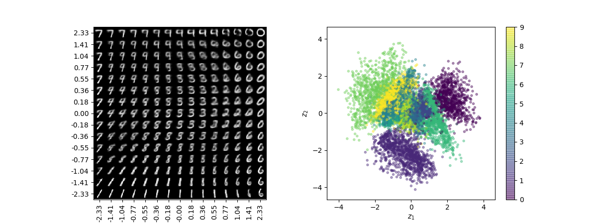
The main issues here are that:

1. Different items can be represented over varying areas in the latent space.
2. No inherent symmetry in the distribution of points.
3. Can be a large separation between items with few samples present during training.

With these in mind:

1. Firstly when it comes to sampling if you pick points uniformly you might be more likely to sample something that ends up decoding to an particular item because the part of the latent space that contained that item during training was larger.
2. Secondly, no obvious way has been set as to how we should randomly select points within our latent space since no distribution has been defined.
3. Thirdly, depending on the encodings generated in training large parts of the latent space would be void of any examples (near the edges perhaps). Autoencoder doesn’t enforce anything when it comes to ensuring that points decoded here are decoded to anything recognizable.
4. Finally, relating to the above since nothing enforces the continuity of the latent space there are no guarantees by slightly adding a small increment to an embedding vector would result in an equally satisfactory item.
   • This issue is subtle in the $2D$ latent space scenario but has the dimensions increase this issue becomes more pronounced.

Resolving Autoencoder Problem: Introducing the Variational Autoencoder (VAE)

In essence what Variational Autoencoders (VAE) do is instead of creating a single point in latent space where an item is embedded into you create a mean and (log) variance vector which become the parameters of a multivariate distribution (normal) which you can then sample from.

To put this more formally the encoder generates vectors $z_{\text{mean}}$ representing the distribution mean across the dimensions and $z_{\text{logvar}}$ representing $\log (\sigma^2)$.

Note: The reason for using the $\log$ function is since by default the variance always has a positive range where as by apply the logarithm the variance can take any real number i.e. $\log {\sigma^2} \in (-\infty, +\infty)$.

Sampling from this works like

\[z = z_{\text{mean}} + \epsilon z_{\text{sigma}}\]

where $\epsilon$ is sampled from the multivariate standard normal distribution. This makes use of the reparameterisation trick which is important since it means you can backpropagate the gradient through the layers freely meaning the partial derivatives can be shown to be deterministic (independent of the random epsilon) which is necessary for back propagation to work.

Maths: Normal Distribution + KL divergence loss

A univariate normal distribution, often simply called a normal distribution, is defined by it’s probability density function (PDF) as:

\[f(x) = \frac{1}{\sqrt{2\pi\sigma^2}} \exp\left( -\frac{(x-\mu)^2}{2\sigma^2} \right)\]

where:

• $x$ is a real-valued random variable.
• $\mu$ is the mean or expectation of the distribution.
• $\sigma$ is the standard deviation.
• $\sigma^2$ is the variance.

A multivariate normal distribution is a generalization of the univariate normal distribution to higher dimensions. Its PDF is given by:

\[f(\mathbf{x}) = \frac{1}{\sqrt{(2\pi)^k |\Sigma|}} \exp\left( -\frac{1}{2} (\mathbf{x}-\mathbf{\mu})^T \Sigma^{-1} (\mathbf{x}-\mathbf{\mu}) \right)\]

where:

• $ \mathbf{x}$ is a $k$-dimensional real vector.
• $\mathbf{\mu}$ is the mean vector.
• $\Sigma$ is the covariance matrix.
• $\lvert \Sigma \rvert$ is the determinant of the covariance matrix.
• $^T$ denotes the transpose of a vector or a matrix.

A special case of these the multivariate standard normal distribution $\mathcal{N}(\mathbb{0},\mathbb{I})$ where $\mathbb{0}$ is the zero valued mean vector and $\mathbb{I}$ is the identity covariance matrix.

Now when it comes to the Kullback-Leibler (KL) divergence loss for we have the form:

\[\begin{align} D_{KL}(P || Q) &= \sum_{i} P(i) \log \frac{P(i)}{Q(i)} \\ D_{KL}\left[N(\mu, \sigma) || N(0, 1)\right] &= \frac{1}{2}\sum_{i}(\mu^{2} + \sigma^{2} + k - \log(\sigma^{2})) \end{align}\]

where $P$ and $Q$ are your two distributions you want to measure divergence between and $k$ represents the dimensionailty of your multivariate normal distribution.

Note: The last equation can be derived from the first by considering the divergence between our two multivariate normal distributions ($P$ being the learned distribution and $Q$ is the standard normal). You can then substtitute in the respective probability density functions and simplify utilising some our the assumptions (covariance matrix is diagonal etc) to get the end result.

Coding up a VAE

The code is relatively similiar when compared with the traditional autoencoder however a few notable differences are present:

1. Encoder logic change
   • A new custom layer will need to be implemented which performs the sampling procedure as described.
   • Additional layers included to handle the fact that the 2 vectors are being outputed.
2. Training loss alteration
   • An additional KL divergence term needs to be added to measure how the probability distrubtions differ from standard normal distribution.
     • In short, the KL divergence term is necessary because it helps in regularizing the latent space to follow a standard normal distribution, aiding in the generative process rather than just learning the compressed representation (is the case when solely using the reconstrcution loss).
     • Without this term, the VAE might learn a complex or even degenerate distribution over the latent space, which would make it difficult to generate new samples.

import tensorflow as tf

class Sampling(tf.keras.layers.Layer):
    def call(self, inputs):
        """
        Implements the reparameterization sampling trick operations for our VAE

        Parameters
        ----------
        inputs : list
            List containing the z_mean and z_log_var vectors outputted from our encoder
        
        Returns
        -------
        Sampled output from distribution
        """
        # Unpacking our two vectors from list
        z_mean, v_log_var = inputs

        # Getting key properties of our vectors
        # Equally could have used the z_log_var
        batch = tf.shape(z_mean)[0]
        dim = tf.shape(z_mean)[1]
        
        # Sampling from our standardised normal distribution
        # Matching shape to that of our vectors
        epsilon = tf.keras.beackend.random_normal(shape=(batch, dim))

        return z_mean + epsilon * tf.exp(0.5 * z_log_var)

# Encoder
encoder_input = tf.keras.layers.Input(
    shape=(IMAGE_SIZE, IMAGE_SIZE, 1), name="encoder_input"
)
x = tf.keras.layers.Conv2D(32, (3, 3), strides=2, activation="relu", padding="same")(
    encoder_input
)
x = tf.keras.layers.Conv2D(64, (3, 3), strides=2, activation="relu", padding="same")(x)
x = tf.keras.layers.Conv2D(128, (3, 3), strides=2, activation="relu", padding="same")(x)
shape_before_flattening = tf.keras.backend.int_shape(x)[1:]  # the decoder will need this!
x = tf.keras.layers.Flatten()(x)

# Generating both our distribution parameter vectors 
z_mean = tf.keras.layers.Dense(EMBEDDING_DIM, name="z_mean")(x)
z_log_var = tf.keras.layers.Dense(EMBEDDING_DIM, name="z_log_var")(x)
# Applying our custom output layer
z = Sampling()([z_mean, z_log_var])

encoder = models.Model(encoder_input, [z_mean, z_log_var, z], name="encoder")
encoder.summary()

# Decoder
decoder_input = tf.keras.layers.Input(shape=(EMBEDDING_DIM,), name="decoder_input")
x = tf.keras.layers.Dense(np.prod(shape_before_flattening))(decoder_input)
x = tf.keras.layers.Reshape(shape_before_flattening)(x)
x = tf.keras.layers.Conv2DTranspose(
    128, (3, 3), strides=2, activation="relu", padding="same"
)(x)
x = tf.keras.layers.Conv2DTranspose(
    64, (3, 3), strides=2, activation="relu", padding="same"
)(x)
x = tf.keras.layers.Conv2DTranspose(
    32, (3, 3), strides=2, activation="relu", padding="same"
)(x)
decoder_output = tf.keras.layers.Conv2D(
    1,
    (3, 3),
    strides=1,
    activation="sigmoid",
    padding="same",
    name="decoder_output",
)(x)

decoder = tf.keras.models.Model(decoder_input, decoder_output)
decoder.summary()

class VAE(models.Model):
    def __init__(self, encoder, decoder, **kwargs):
        super(VAE, self).__init__(**kwargs)
        self.encoder = encoder
        self.decoder = decoder
        self.total_loss_tracker = metrics.Mean(name="total_loss")
        self.reconstruction_loss_tracker = metrics.Mean(
            name="reconstruction_loss"
        )
        self.kl_loss_tracker = metrics.Mean(name="kl_loss")

    @property
    def metrics(self):
        return [
            self.total_loss_tracker,
            self.reconstruction_loss_tracker,
            self.kl_loss_tracker,
        ]

    def call(self, inputs):
        """Call the model on a particular input."""
        z_mean, z_log_var, z = encoder(inputs)
        reconstruction = decoder(z)
        return z_mean, z_log_var, reconstruction

    def train_step(self, data):
        """Step run during training."""
        with tf.GradientTape() as tape:
            z_mean, z_log_var, reconstruction = self(data)
            reconstruction_loss = tf.reduce_mean(
                BETA
                * losses.binary_crossentropy(
                    data, reconstruction, axis=(1, 2, 3)
                )
            )
            kl_loss = tf.reduce_mean(
                tf.reduce_sum(
                    -0.5
                    * (1 + z_log_var - tf.square(z_mean) - tf.exp(z_log_var)),
                    axis=1,
                )
            )
            total_loss = reconstruction_loss + kl_loss

        grads = tape.gradient(total_loss, self.trainable_weights)
        self.optimizer.apply_gradients(zip(grads, self.trainable_weights))

        self.total_loss_tracker.update_state(total_loss)
        self.reconstruction_loss_tracker.update_state(reconstruction_loss)
        self.kl_loss_tracker.update_state(kl_loss)

        return {m.name: m.result() for m in self.metrics}

    def test_step(self, data):
        """Step run during validation."""
        if isinstance(data, tuple):
            data = data[0]

        z_mean, z_log_var, reconstruction = self(data)
        reconstruction_loss = tf.reduce_mean(
            BETA
            * tf.keras.losses.binary_crossentropy(data, reconstruction, axis=(1, 2, 3))
        )
        kl_loss = tf.reduce_mean(
            tf.reduce_sum(
                -0.5 * (1 + z_log_var - tf.square(z_mean) - tf.exp(z_log_var)),
                axis=1,
            )
        )
        total_loss = reconstruction_loss + kl_loss

        return {
            "loss": total_loss,
            "reconstruction_loss": reconstruction_loss,
            "kl_loss": kl_loss,
        }

# Creating a vae object
vae = VAE(encoder, decoder)

where for the encoder:

• encoder_input = tf.keras.layers.Input(shape=(IMAGE_SIZE, IMAGE_SIZE, 1), name="encoder_input"):
  • This line is defining the input to the encoder, which is an image of size IMAGE_SIZE x IMAGE_SIZE with one channel (for grayscale images).
• x = tf.keras.layers.Conv2D(32, (3, 3), strides=2, activation="relu", padding="same")(encoder_input):
  • This line adds a 2D convolution layer to the model. The layer has 32 filters, each of which is a 3x3 square. The stride of 2 means that the filters move two pixels at a time, reducing the size of the image. The ReLU activation function introduces non-linearity into the model, and ‘same’ padding means that zeros are added around the input image so that the convolution operation does not reduce the image size.
• The following two lines add additional 2D convolution layers, each with more filters than the last (64 and 128 respectively).
  • This allows the model to learn more complex representations.
• shape_before_flattening = tf.keras.backend.int_shape(x)[1:]:
  • This line is used to store the shape of the tensor before it is flattened, which will be useful when we want to reshape it back in the decoder.
• x = tf.keras.layers.Flatten()(x):
  • This line flattens the tensor to a vector, which is necessary because the next layer (the Dense layer) expects its input in this format.
• z_mean = tf.keras.layers.Dense(EMBEDDING_DIM, name="z_mean")(x) and z_log_var = tf.keras.layers.Dense(EMBEDDING_DIM, name="z_log_var")(x):
  • These lines define two Dense layers that output the parameters (mean and log variance) of the distribution in the latent space.
• z = Sampling()([z_mean, z_log_var]):
  • This line applies a custom Sampling layer to the z_mean and z_log_var. This Sampling layer is what was defined separatly and it is responsible for generating a point in the latent space by sampling from the distribution defined by z_mean and z_log_var.
• encoder = tf.keras.models.Model(encoder_input, [z_mean, z_log_var, z], name="encoder"):
  • This line defines the encoder model, specifying the input and output tensors.
• encoder.summary():
  • This line prints a summary of the encoder model, including the number of parameters and the output shapes of each layer.

where for the decoder:

• decoder_input = tf.keras.layers.Input(shape=(EMBEDDING_DIM,), name="decoder_input"): This line defines the input to the decoder, which is a point in the latent space. The shape of this point is (EMBEDDING_DIM,).
• x = tf.keras.layers.Dense(np.prod(shape_before_flattening))(decoder_input):
  • This line creates a Dense layer (fully connected layer) that takes the decoder input and outputs a vector of size equal to the product of the dimensions of shape_before_flattening. This is the shape stored from the last convolutional layer in the encoder before flattening.
• x = tf.keras.layers.Reshape(shape_before_flattening)(x):
  • This line reshapes the vector back to its original dimensions before it was flattened in the encoder. This is necessary because the next layer (a Conv2DTranspose layer) expects its input in this format.
• The next three lines add Conv2DTranspose layers (also known as deconvolutional layers or fractionally-strided convolutions) to the model.
  • These layers perform the inverse operation of a Conv2D layer: they increase the size of the image rather than reducing it. They do this by padding the input in such a way that a regular convolution produces an output of larger size. In this case, the Conv2DTranspose layers have 128, 64, and 32 filters respectively, and each uses a stride of 2 to double the size of the image at each step.
  • The ReLU activation function introduces non-linearity into the model, and ‘same’ padding means that the convolution operation maintains the image size.
• decoder_output = tf.keras.layers.Conv2D(1, (3, 3), strides=1, activation="sigmoid", padding="same", name="decoder_output")(x):
  • This line defines the final layer of the decoder, which is a Conv2D layer with a single filter. The output of this layer is an image of the same size as the input to the decoder. The sigmoid activation function is used to ensure that the output values are between 0 and 1, which is necessary because the input images are assumed to be normalized in this range.
• decoder = tf.keras.models.Model(decoder_input, decoder_output):
  • This line defines the decoder model, specifying the input and output tensors.
• decoder.summary():
  • This line prints a summary of the decoder model, including the number of parameters and the output shapes of each layer.

and finally for the final model class:

• def __init__(self, encoder, decoder, **kwargs):
  • The constructor method takes an encoder and a decoder (which are themselves models), and optionally any number of additional keyword arguments. It initializes the VAE by calling the base class constructor and storing the encoder and decoder as instance variables. It also creates three metrics.
  • Mean objects to keep track of the total loss, the reconstruction loss, and the KL divergence loss over an epoch.
• @property def metrics(self):
  • This method is a property that returns a list of the metrics to be tracked.
  • The @property decorator allows us to use it like a regular instance attribute (i.e., vae.metrics) instead of a method.
• def call(self, inputs):
  • This method is used to compute the forward pass of the model. Given an input, it computes the encoded representation (mean, log variance, and sampled point in the latent space) and then the decoded reconstruction.
• def train_step(self, data):
  • This method is called once per batch during training. It performs the forward pass, computes the losses, computes the gradients of the losses with respect to the model’s trainable weights, and updates the weights using the optimizer. It also updates the state of the loss trackers.
• def test_step(self, data):
  • This method is called once per batch during evaluation. It performs the forward pass, computes the losses, and returns them in a dictionary.
• The losses are computed as discussed above
  • reconstruction_loss:
    • This is the binary cross-entropy loss between the input data and the reconstruction. It is scaled by a factor BETA, which could be used to balance the importance of the reconstruction loss and the KL divergence loss.
  • kl_loss:
    • This is the Kullback-Leibler divergence, which measures the difference between the learned latent distribution and a standard normal distribution.
  • total_loss:
    • This is the sum of the reconstruction loss and the KL divergence loss.
• The train_step and test_step methods are used when you want to customize the training and testing loops.
  • In short, you only need to implement and call these methods if you are customizing the training or evaluation process beyond what the standard fit and evaluate methods provide.
  • In the case of the Variational Autoencoder (VAE) class, the train_step and test_step methods are overridden to calculate and apply the specific losses that VAEs use: the reconstruction loss and the Kullback-Leibler (KL) divergence loss for training and testing.

Real World Usecases

Leading on from the original defintion of autoencoders that we went over intially it can seem somewhat obvious that many use cases can stem from them all which in some form or another revolve around understanding your input data and creating a nice representation.

Here is a non-exhaustive list of a few:

1. Image Denoising: Autoencoders can be used to remove noise from images. The idea is to train the autoencoder with noisy images as input and the corresponding clean images as output. Once trained, it can denoise other noisy images effectively.
2. Anomaly Detection: Autoencoders can be used for anomaly detection, especially in time-series data. For example, they can be trained on normal operations data from a machine, and can then be used to detect deviations from the normal, signaling potential faults or failures.
3. Feature Learning: Autoencoders, especially convolutional autoencoders, can be used to learn compressed feature representations of data. These features can then be used in other machine learning tasks.
4. Data Visualization: Autoencoders can be used for dimensionality reduction similar to PCA (Principal Component Analysis) or t-SNE, allowing for the visualization of high-dimensional data in 2D or 3D space.
5. Image Compression: Autoencoders can be trained to reduce the dimensionality of images, effectively compressing them. The decoder can then be used to reconstruct the original image from the compressed representation.
6. Generating Art: Variational autoencoders (VAEs) are a special kind of autoencoder that can generate new instances that are similar to your input data. They can be used to generate art based on a dataset of existing art pieces.
7. Data Generation and Augmentation: Autoencoders, especially VAEs, can be used to generate new data samples that are similar to the training data. This can be particularly useful for augmenting datasets in situations where collecting more real data is challenging or expensive.
8. Recommendation Systems: Autoencoders can be used to learn the underlying structure of user-item interaction data, and can be useful in building recommendation systems. For instance, training an autoencoder on user ratings can help in predicting missing ratings.
9. Sequential Data Processing: Sequence-to-sequence autoencoders can be used to process and generate sequential data, making them useful for tasks like machine translation, and time-series forecasting.
10. Drug Discovery: Autoencoders can be used in the field of bioinformatics and drug discovery. By training on molecular data, they can aid in generating potential new drug compounds.
11. Removing Watermarks: While this can be a controversial application that I myself don’t endorse 😑, autoencoders can be trained to remove watermarks or other artifacts from images.
12. Face Recognition and Modification: Autoencoders can be trained to recognize facial features and can be used for tasks like face swapping, age progression/regression, or changing facial expressions.

Alot of these span across various domains both with respects to business and AI. Here are a few posts which show case these additionally, 7 applications of autoecnoders Medium article and working with autoencoders NeptuneAI blog

Resources

• Papers
  • Intro to Variational Autoencoders
    • Paper released in 2019 summarising VAEs and some extenstions.
    • Written by folks at Google.
  • Masked Autoencoders in Computer Vision
    • Interesting application of autoencoders.
• Posts/blogs/articles
  • Origins of Autoencoders
    • Q&A post about the origins of autoencoders.
    • Seems that they date as far back as the 1980/90s.
  • TensorFlow Autoencoder Tutorial
    • Tutorial walkthrough on using autoencoders with TensorFlow.

Citation Information

If you find this content useful & plan on using it, please consider citing it using the following format:

@misc{nish-blog,
  title = {Autoencoders Explained - Breathing Life into Data},
  author = {Nish},
  howpublished = {\url{https://www.nishbhana.com/Autoencoders/}},
  note = {[Online; accessed]},
  year = {2023}
}

Share: x.com, Facebook